Introduction

Motivation

Shiny apps are a wonderful way to communicate data to others. It allows for interactivity to get additional insights into the data without completely re-running an analysis and re-generating a report.

Within the OHDSI sphere it is customary that a study has a accompanying shiny app, to visualize the data. OhdsiShinyModules and ShinyAppBuilder were developed to standardize shiny apps for commonly ran analyses, mainly from the HADES suite.

ShinyAppBuilder seems to be air tight in the way it functions, without much room for flexibility. It has to, to maintain the level of standardization it provides. It offers the most extreme opposite of what developing a fully customized shiny app would be.

DarwinShinyModules attempts to strike the middle ground between both. It deals with the overhead of shiny, like namespaces, reactive environments, and server execution; provides pre-specified modules to rapidly develop functional shiny apps, but stays flexible enough to include custom additions to your shiny app.

Kinds of modules

The idea behind DarwinShinyModules is that one component can be a module. A component may be a plot, a table, text, etc. These kinds of modules contain code to deal with some kind of data, and present the output in a standardized way. For instance a Table module might show a form of tabular data like a data.frame the same standardizes way, independent of the contents of the data.

As an example we can display the contents of the iris and mtcars data sets in a similar fashion:

library(DarwinShinyModules)

tableIris <- Table$new(iris, title = "Iris")
tableMtcars <- Table$new(mtcars, title = "MT Cars")

preview(list(tableIris, tableMtcars))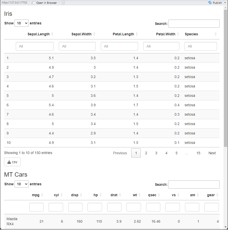

Shiny applications not supported in static R Markdown documents

Notice that both tables are effectively formatted the same, and that only the data contained within is different. Both have a button to download the visualized data in the bottom left, both are search-able per column, etc.

We will call modules that deal directly with data like this base modules. These modules are the lowest level of module there is when building other modules or shiny apps. These modules can be directly used in any form of shiny app, or other module.

The second kind of module in DarwinShinyModules is a composed module. This kind of module is a for a large part of its server code composed of other modules. Additional code can make it so these modules can communicate with each other.

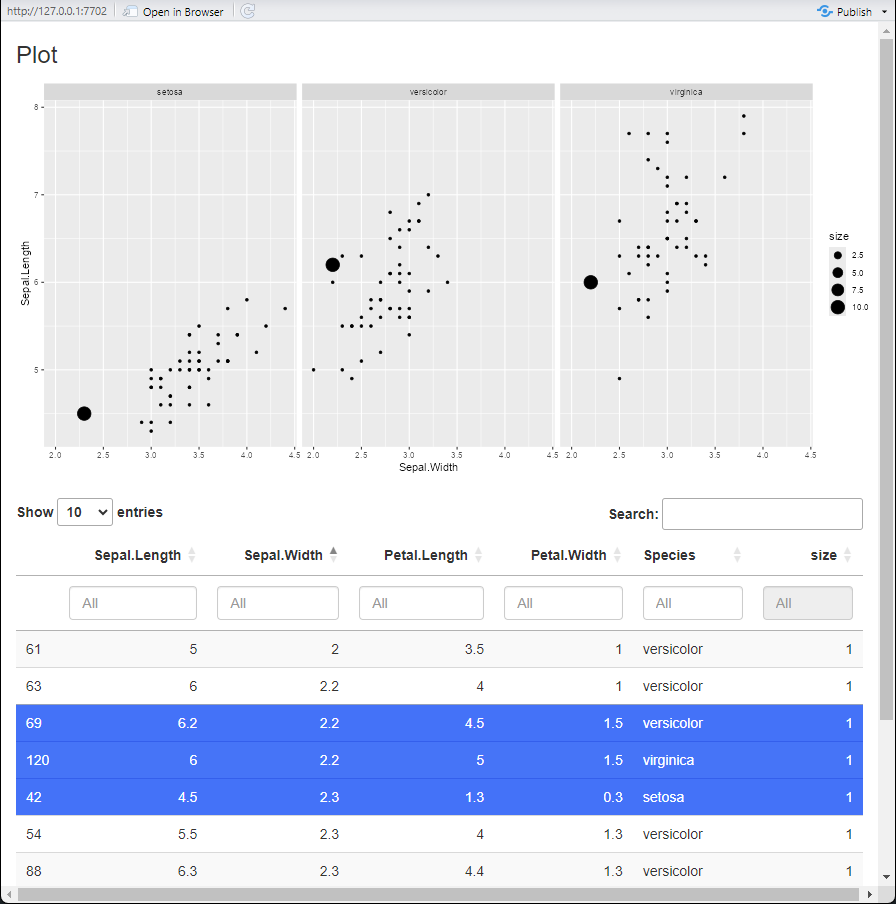
As an example, this server function uses the pre-specified table and plot server methods. A small amount of code is then added to update a “size” column in the data, depending on what rows are selected in the table, and then updated in the plot. The plot will then update with the updated data.

server = function(input, output, session) {
  # Server method for the `plot`
  private$.plot$server(input, output, session)
  # Server method for the `table`
  private$.table$server(input, output, session)

  # Additional code that fetches `rows_selected` from the `table` module, and
  # uses it to update the data in the `plot` module
  shiny::observeEvent(private$.table$bindings$rows_selected, {
    private$.data[, "size"] <- 1
    private$.data[private$.table$bindings$rows_selected, "size"] <- 10
    private$.plot$args$data <- private$.data
  })
}

The full underlying code is out of scope of this vignette, but included at the end of this vignette for completeness in supplementary A.

Module hierarchy

Now that we know what kind of modules we have, we can explore the hierarchy of modules. DarwinShinyModules uses R6 to implement each module. Even though R is a functional language and does not inherently support Object Oriented Programming (OOP), this style of code organisation lends itself very well to create shiny modules and gives a sense of “state” within each module. This “state” can then be manipulated during run time depending on user input, changing the behavior of (other) modules dynamically.

A sense of “state” is also achievable with purely functions, and functional programming but the data is has to live in either the global environment, on disk, or the data needs to be attached to a function environment:

foo <- function(x) {
  z <- x

  function(y) {
    z * y
  }
}

bar <- foo(2)

bar(3)
#> [1] 6

All of these options seem like a more round about way of doing things, for this use case.

DarwinShinyModules uses inheritance to inherit common functionality between modules, following a “decorator” style design pattern. The idea behind this is that inheritance should come naturally, and (hopefully) intuitively.

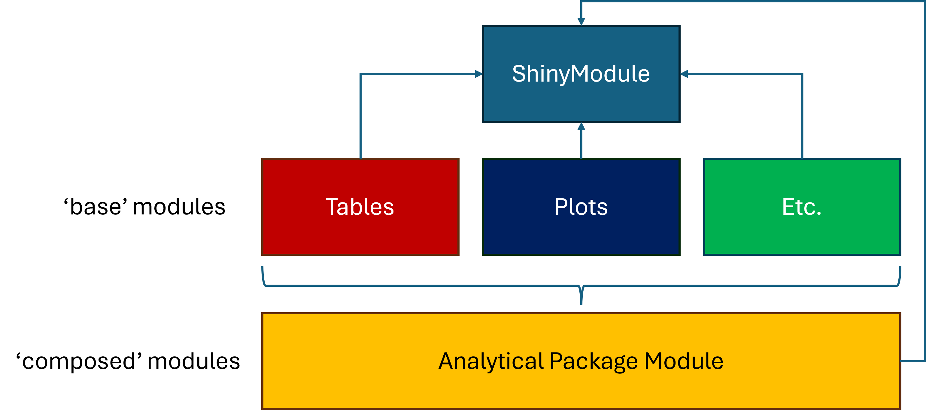
At the top of this hierarchy is the ShinyModule class. This class deals with the overhead of shiny, like namespaces, reactive environments, and server execution. All other modules in DarwinShinyModules inherit from this module. The second layer of modules are the ‘base’ modules described earlier. Some of these modules might have an intermediate parent class. For instance the PlotStatic, PlotWidget, and PlotPlotly inherit from a Plot class. This is mostly due to the specific renderX() and XOutput() functions specific for each kind of plot. Finally in the third layer are the ‘composed’ modules.

Suplementals

A: Full code

ExampleModule <- R6::R6Class(
  classname = "ExampleModule",
  inherit = ShinyModule,
  
  active = list(),
  public = list(
    initialize = function() {
      super$initialize()
      private$.data <- iris
      private$.data$size <- 1
      private$.table <- Table$new(private$.data, title = NULL)
      private$.table$parentNamespace <- self$namespace
      
      private$.plot <- PlotStatic$new(fun = private$.plotFun, args = list(data = private$.data))
      private$.plot$parentNamespace <- self$namespace
    }
  ),
  private = list(
    .data = NULL,
    .table = NULL,
    .plot = NULL,
    
    .UI = function() {
      shiny::tagList(
        private$.plot$UI(),
        private$.table$UI()
      )
    },
    
    .server = function(input, output, session) {
      private$.plot$server(input, output, session)
      private$.table$server(input, output, session)

      shiny::observeEvent(private$.table$bindings$rows_selected, {
        private$.data[, "size"] <- 1
        private$.data[private$.table$bindings$rows_selected, "size"] <- 10
        private$.plot$args$data <- private$.data
      })
    },
    
    .plotFun = function(data) {
      ggplot2::ggplot(data = data) +
        ggplot2::geom_point(mapping = ggplot2::aes(x = Sepal.Width, y = Sepal.Length, size = size)) +
        ggplot2::facet_grid(. ~ Species)
    }
  )
)

mod <- ExampleModule$new()
preview(mod)