The Observational Medical Outcomes Partnership (OMOP) Common Data Model (CDM) is a commonly used format for storing and analyzing observational health data derived from electronic health records, insurance claims, registries, and other sources. Source data is “mapped” into the OMOP CDM format providing researchers with a standardized interface for querying and analyzing observational health data. The CDMConnector package provides tools for working with OMOP Common Data Model (CDM) tables using familiar dplyr syntax and using the tidyverse design principles popular in the R ecosystem.
This vignette is for new users of CDMConnector who have access to data already mapped into the OMOP CDM format. However, CDMConnector does provide several example synthetic datasets in the OMOP CDM format. To learn more about the OMOP CDM or the mapping process check out these resources.
Creating a reference to the OMOP CDM
Typically OMOP CDM datasets are stored in a database and can range in size from hundreds of patients with thousands of records to hundreds of millions of patients with billions of records. The Observational Health Data Science and Informatics (OHDSI) community supports a selection of popular database platforms including Postgres, Microsoft SQL Server, Oracle, as well as cloud data platforms such as Amazon Redshift, Google Big Query, Databricks, and Snowflake. The first step in using CDMConnector is to create a connection to your database from R. This can take some effort the first time you set up drivers. See the “Database Connection Examples” vignette or check out the Posit’s database documentation.
In our example’s we will use some synthetic data from the Synthea project
that has been mapped to the OMOP CDM format. We’ll use the duckdb database which is a file based
database similar to SQLite but with better date type support. To see all
the example datasets available run exampleDatasets().
library(CDMConnector)
exampleDatasets()
#>  [1] "GiBleed"                             "synthea-allergies-10k"
#>  [3] "synthea-anemia-10k"                  "synthea-breast_cancer-10k"
#>  [5] "synthea-contraceptives-10k"          "synthea-covid19-10k"
#>  [7] "synthea-covid19-200k"                "synthea-dermatitis-10k"
#>  [9] "synthea-heart-10k"                   "synthea-hiv-10k"
#> [11] "synthea-lung_cancer-10k"             "synthea-medications-10k"
#> [13] "synthea-metabolic_syndrome-10k"      "synthea-opioid_addiction-10k"
#> [15] "synthea-rheumatoid_arthritis-10k"    "synthea-snf-10k"
#> [17] "synthea-surgery-10k"                 "synthea-total_joint_replacement-10k"
#> [19] "synthea-veteran_prostate_cancer-10k" "synthea-veterans-10k"
#> [21] "synthea-weight_loss-10k"             "synpuf-1k"
#> [23] "synpuf-110k"                         "empty_cdm"
#> [25] "Synthea27NjParquet"                  "delphi-100k"

con <- DBI::dbConnect(duckdb::duckdb(), eunomiaDir("GiBleed"))
DBI::dbListTables(con)
#>  [1] "care_site"             "cdm_source"            "concept"
#>  [4] "concept_ancestor"      "concept_class"         "concept_relationship"
#>  [7] "concept_synonym"       "condition_era"         "condition_occurrence"
#> [10] "cost"                  "death"                 "device_exposure"
#> [13] "domain"                "dose_era"              "drug_era"
#> [16] "drug_exposure"         "drug_strength"         "fact_relationship"
#> [19] "location"              "measurement"           "metadata"
#> [22] "note"                  "note_nlp"              "observation"
#> [25] "observation_period"    "payer_plan_period"     "person"
#> [28] "procedure_occurrence"  "provider"              "relationship"
#> [31] "source_to_concept_map" "specimen"              "visit_detail"
#> [34] "visit_occurrence"      "vocabulary"
If you’re using CDMConnector for the first time you may get a message
about adding an environment variable EUNOMIA_DATA_FOLDER .
To do this simply create a new text file in your home directory called
.Renviron and add the line
EUNOMIA_DATA_FOLDER="path/to/folder/where/we/can/store/example/data".
If you run usethis::edit_r_environ() this file will be
created and opened for you and opened in RStudio.
After connecting to a database containing data mapped to the OMOP
CDM, use cdmFromCon to create a CDM reference. This CDM
reference is a single object that contains dplyr table references to
each CDM table along with metadata about the CDM instance.
The cdmSchema is the schema in the database that
contains the OMOP CDM tables and is required. The
writeSchema is a schema in the database where the user has
the ability to create tables. Both cdmSchema and
writeSchema are required to create a cdm object.
Every cdm object needs a cdmName that is used to
identify the CDM in output files.
cdm <- cdmFromCon(con, cdmName = "eunomia", cdmSchema = "main", writeSchema = "main")
cdm
#>
#> ── # OMOP CDM reference (duckdb) of eunomia ────────────────────────────────────
#> • omop tables: care_site, cdm_source, concept, concept_ancestor, concept_class,
#> concept_relationship, concept_synonym, condition_era, condition_occurrence,
#> cost, death, device_exposure, domain, dose_era, drug_era, drug_exposure,
#> drug_strength, fact_relationship, location, measurement, metadata, note,
#> note_nlp, observation, observation_period, payer_plan_period, person,
#> procedure_occurrence, provider, relationship, source_to_concept_map, specimen,
#> visit_detail, visit_occurrence, vocabulary
#> • cohort tables: -
#> • achilles tables: -
#> • other tables: -
cdm$observation_period
#> # Source: table<observation_period> [?? x 5]
#> # Database: DuckDB 1.4.4 [root@Darwin 25.3.0:R 4.5.1//private/var/folders/2j/8z0yfn1j69q8sxjc7vj9yhz40000gp/T/RtmprYE29l/file108368bccd5b.duckdb]
#> observation_period_id person_id observation_period_s…¹ observation_period_e…²
#> <int> <int> <date> <date>
#> 1 6 6 1963-12-31 2007-02-06
#> 2 13 13 2009-04-26 2019-04-14
#> 3 27 27 2002-01-30 2018-11-21
#> 4 16 16 1971-10-14 2017-11-02
#> 5 55 55 2009-05-30 2019-03-23
#> 6 60 60 1990-11-21 2019-01-23
#> 7 42 42 1909-11-03 2019-03-13
#> 8 33 33 1986-05-12 2018-09-10
#> 9 18 18 1965-11-17 2018-11-07
#> 10 25 25 2007-03-18 2019-04-07
#> # ℹ more rows
#> # ℹ abbreviated names: ¹observation_period_start_date,
#> # ²observation_period_end_date
#> # ℹ 1 more variable: period_type_concept_id <int>Individual CDM table references can be accessed using `$`.
cdm$person %>%
  dplyr::glimpse()
#> Rows: ??
#> Columns: 18
#> Database: DuckDB 1.4.4 [root@Darwin 25.3.0:R 4.5.1//private/var/folders/2j/8z0yfn1j69q8sxjc7vj9yhz40000gp/T/RtmprYE29l/file108368bccd5b.duckdb]
#> $ person_id                   <int> 6, 123, 129, 16, 65, 74, 42, 187, 18, 111,…
#> $ gender_concept_id           <int> 8532, 8507, 8507, 8532, 8532, 8532, 8532, …
#> $ year_of_birth               <int> 1963, 1950, 1974, 1971, 1967, 1972, 1909, …
#> $ month_of_birth              <int> 12, 4, 10, 10, 3, 1, 11, 7, 11, 5, 8, 3, 3…
#> $ day_of_birth                <int> 31, 12, 7, 13, 31, 5, 2, 23, 17, 2, 19, 13…
#> $ birth_datetime              <dttm> 1963-12-31, 1950-04-12, 1974-10-07, 1971-…
#> $ race_concept_id             <int> 8516, 8527, 8527, 8527, 8516, 8527, 8527, …
#> $ ethnicity_concept_id        <int> 0, 0, 0, 0, 0, 0, 0, 0, 0, 0, 0, 0, 0, 0, …
#> $ location_id                 <int> NA, NA, NA, NA, NA, NA, NA, NA, NA, NA, NA…
#> $ provider_id                 <int> NA, NA, NA, NA, NA, NA, NA, NA, NA, NA, NA…
#> $ care_site_id                <int> NA, NA, NA, NA, NA, NA, NA, NA, NA, NA, NA…
#> $ person_source_value         <chr> "001f4a87-70d0-435c-a4b9-1425f6928d33", "0…
#> $ gender_source_value         <chr> "F", "M", "M", "F", "F", "F", "F", "M", "F…
#> $ gender_source_concept_id    <int> 0, 0, 0, 0, 0, 0, 0, 0, 0, 0, 0, 0, 0, 0, …
#> $ race_source_value           <chr> "black", "white", "white", "white", "black…
#> $ race_source_concept_id      <int> 0, 0, 0, 0, 0, 0, 0, 0, 0, 0, 0, 0, 0, 0, …
#> $ ethnicity_source_value      <chr> "west_indian", "italian", "polish", "ameri…
#> $ ethnicity_source_concept_id <int> 0, 0, 0, 0, 0, 0, 0, 0, 0, 0, 0, 0, 0, 0, …
You can then use dplyr to query the cdm tables just as you would an R
dataframe. The difference is that the data stays in the database and SQL
code is dynamically generated and set to the database backend. The goal
is to allow users to not think too much about the database or SQL and
instead use familiar R syntax to work with these large tables.
collect will bring the data from the database into R. Be
careful not to request a gigantic result set! In general it is better to
aggregate data in the database, if possible, before bringing data into
R.
library(dplyr)
#>
#> Attaching package: 'dplyr'
#> The following objects are masked from 'package:stats':
#>
#>     filter, lag
#> The following objects are masked from 'package:base':
#>
#>     intersect, setdiff, setequal, union
library(ggplot2)

cdm$person %>%
  group_by(year_of_birth, gender_concept_id) %>%
  summarize(n = n(), .groups = "drop") %>%
  collect() %>%
  mutate(sex = case_when(
    gender_concept_id == 8532 ~ "Female",
    gender_concept_id == 8507 ~ "Male"
  )) %>%
  ggplot(aes(y = n, x = year_of_birth, fill = sex)) +
  geom_histogram(stat = "identity", position = "dodge") +
  labs(x = "Year of birth",
       y = "Person count",
       title = "Age Distribution",
       subtitle = cdmName(cdm),
       fill = NULL) +
  theme_bw()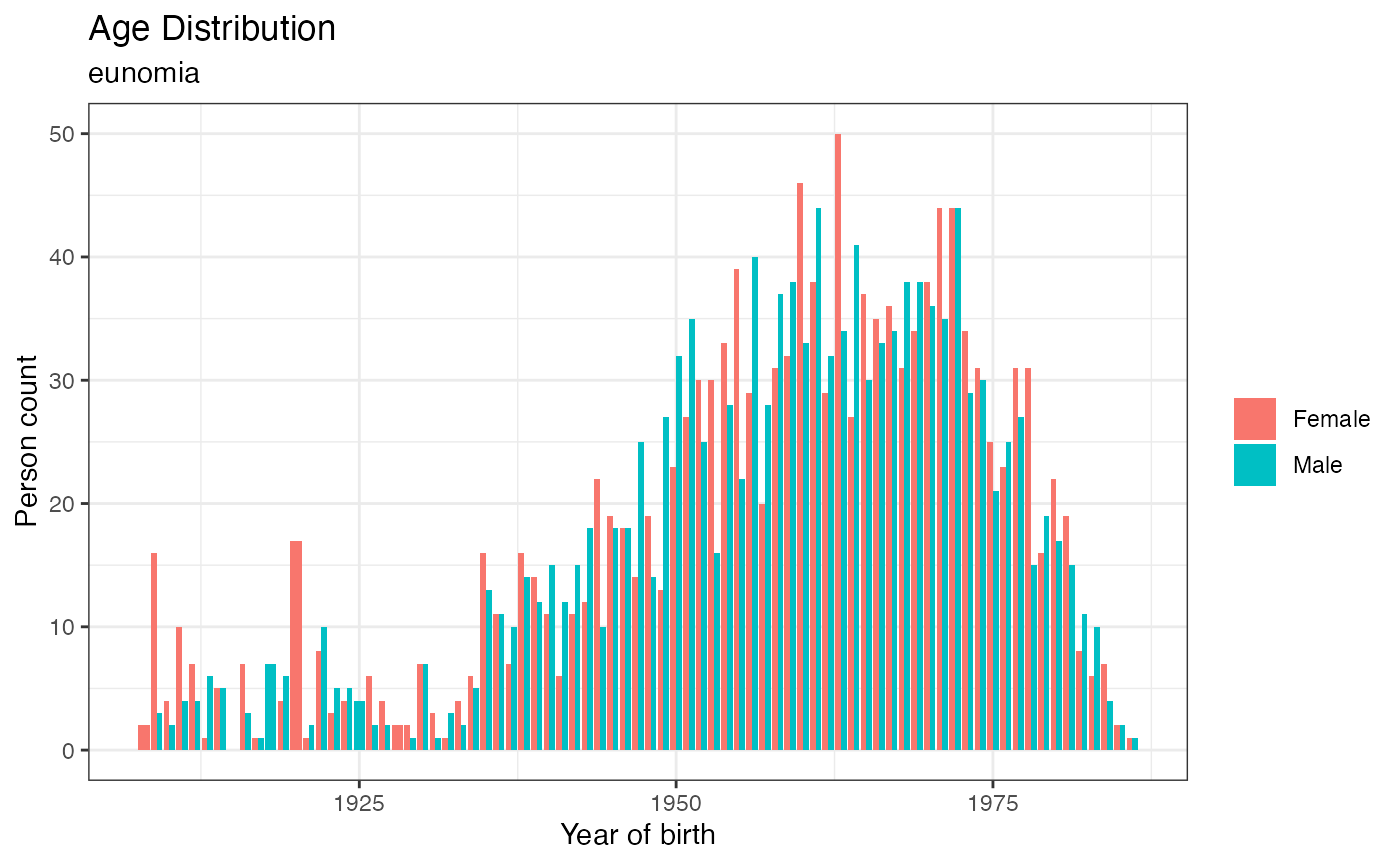
Joining tables
Since the OMOP CDM is a relational data model joins are very common in analytic code. All of the events in the OMOP CDM are recorded using integers representing standard “concepts”. To see the text description of a concept researchers need to join clinical tables to the concept vocabulary table. Every OMOP CDM should have a copy of the vocabulary used to map the data to the OMOP CDM format.
Here is an example query looking at the most common conditions in the CDM.
cdm$condition_occurrence %>%
  count(condition_concept_id, sort = T) %>%
  left_join(cdm$concept, by = c("condition_concept_id" = "concept_id")) %>%
  collect() %>%
  select("condition_concept_id", "concept_name", "n")
#> # A tibble: 80 × 3
#>    condition_concept_id concept_name                                           n
#>                   <int> <chr>                                              <dbl>
#>  1              4116491 Escherichia coli urinary tract infection             482
#>  2              4113008 Laceration of hand                                   500
#>  3              4156265 Facial laceration                                    497
#>  4              4155034 Laceration of forearm                                507
#>  5              4109685 Laceration of foot                                   484
#>  6              4094814 Bullet wound                                          46
#>  7              4048695 Fracture of vertebral column without spinal cord …    23
#>  8             40486433 Perennial allergic rhinitis                           64
#>  9              4051466 Childhood asthma                                      96
#> 10              4142905 Fracture of rib                                      263
#> # ℹ 70 more rows
Let’s look at the most common drugs used by patients with “Acute viral pharyngitis”.
cdm$condition_occurrence %>%
  filter(condition_concept_id == 4112343) %>%
  distinct(person_id) %>%
  inner_join(cdm$drug_exposure, by = "person_id") %>%
  count(drug_concept_id, sort = TRUE) %>%
  left_join(cdm$concept, by = c("drug_concept_id" = "concept_id")) %>%
  collect() %>%
  select("concept_name", "n")
#> # A tibble: 113 × 2
#>    concept_name                                                      n
#>    <chr>                                                         <dbl>
#>  1 hepatitis B vaccine, adult dosage                              1826
#>  2 Alendronic acid 10 MG Oral Tablet                               129
#>  3 alteplase 100 MG Injection                                      210
#>  4 Nitroglycerin 0.4 MG/ACTUAT Mucosal Spray                       207
#>  5 atorvastatin 80 MG Oral Tablet                                   57
#>  6 Fentanyl                                                          8
#>  7 Etonogestrel 68 MG Drug Implant                                   6
#>  8 Galantamine 4 MG Oral Tablet                                     83
#>  9 Levonorgestrel 0.00354 MG/HR Drug Implant                        29
#> 10 {28 (Norethindrone 0.35 MG Oral Tablet) } Pack [Errin 28 Day]     4
#> # ℹ 103 more rows
To inspect the generated SQL use show_query from
dplyr.
cdm$condition_occurrence %>%
  filter(condition_concept_id == 4112343) %>%
  distinct(person_id) %>%
  inner_join(cdm$drug_exposure, by = "person_id") %>%
  count(drug_concept_id, sort = TRUE) %>%
  left_join(cdm$concept, by = c("drug_concept_id" = "concept_id")) %>%
  show_query()
#> <SQL>
#> SELECT
#>   LHS.*,
#>   concept_name,
#>   domain_id,
#>   vocabulary_id,
#>   concept_class_id,
#>   standard_concept,
#>   concept_code,
#>   valid_start_date,
#>   valid_end_date,
#>   invalid_reason
#> FROM (
#>   SELECT drug_concept_id, COUNT(*) AS n
#>   FROM (
#>     SELECT
#>       LHS.person_id AS person_id,
#>       drug_exposure_id,
#>       drug_concept_id,
#>       drug_exposure_start_date,
#>       drug_exposure_start_datetime,
#>       drug_exposure_end_date,
#>       drug_exposure_end_datetime,
#>       verbatim_end_date,
#>       drug_type_concept_id,
#>       stop_reason,
#>       refills,
#>       quantity,
#>       days_supply,
#>       sig,
#>       route_concept_id,
#>       lot_number,
#>       provider_id,
#>       visit_occurrence_id,
#>       visit_detail_id,
#>       drug_source_value,
#>       drug_source_concept_id,
#>       route_source_value,
#>       dose_unit_source_value
#>     FROM (
#>       SELECT DISTINCT person_id
#>       FROM condition_occurrence
#>       WHERE (condition_concept_id = 4112343.0)
#>     ) LHS
#>     INNER JOIN drug_exposure
#>       ON (LHS.person_id = drug_exposure.person_id)
#>   ) q01
#>   GROUP BY drug_concept_id
#> ) LHS
#> LEFT JOIN concept
#>   ON (LHS.drug_concept_id = concept.concept_id)
These are a few simple queries. More complex queries can be built by combining simple queries like the ones above and other analytic packages provide functions that implement common analytic use cases.
For example a “cohort definition” is a set of criteria that persons must satisfy that can be quite complex. The “Working with Cohorts” vignette describes creating and using cohorts with CDMConnector.
Saving query results to the database
Sometimes it is helpful to save query results to the database instead
of reading the result into R. dplyr provides the compute
function but due to differences between database systems CDMConnector
has needed to export its own method that handles the slight differences.
Internally CDMConnector runs compute_query function that is
tested across the OHDSI supported database platforms.
If we are writing data to the CDM database we need to add one more argument when creating our cdm reference object, the “write_schema”. This is a schema in the database where you have write permissions. Typically this should be a separate schema from the “cdm_schema”.
DBI::dbExecute(con, "create schema scratch;")
#> [1] 0
cdm <- cdmFromCon(con, cdmName = "eunomia", cdmSchema = "main", writeSchema = "scratch")
#> Note: method with signature 'DBIConnection#Id' chosen for function 'dbExistsTable',
#>  target signature 'duckdb_connection#Id'.
#>  "duckdb_connection#ANY" would also be valid
drugs <- cdm$condition_occurrence %>%
  filter(condition_concept_id == 4112343) %>%
  distinct(person_id) %>%
  inner_join(cdm$drug_exposure, by = "person_id") %>%
  count(drug_concept_id, sort = TRUE) %>%
  left_join(cdm$concept, by = c("drug_concept_id" = "concept_id")) %>%
  compute(name = "test", temporary = FALSE, overwrite = TRUE)

drugs %>% show_query()
#> <SQL>
#> SELECT *
#> FROM scratch.test

drugs
#> # Source:   table<scratch.test> [?? x 11]
#> # Database: DuckDB 1.4.4 [root@Darwin 25.3.0:R 4.5.1//private/var/folders/2j/8z0yfn1j69q8sxjc7vj9yhz40000gp/T/RtmprYE29l/file108368bccd5b.duckdb]
#>    drug_concept_id     n concept_name   domain_id vocabulary_id concept_class_id
#>              <int> <dbl> <chr>          <chr>     <chr>         <chr>
#>  1        40162522   305 Acetaminophen… Drug      RxNorm        Clinical Drug
#>  2        19133873  1666 Penicillin V … Drug      RxNorm        Clinical Drug
#>  3        40236446    63 Methylphenida… Drug      RxNorm        Clinical Drug
#>  4        19073188   246 Amoxicillin 5… Drug      RxNorm        Clinical Drug
#>  5        40163554   135 Warfarin Sodi… Drug      RxNorm        Clinical Drug
#>  6        19016749    16 remifentanil   Drug      RxNorm        Ingredient
#>  7        46275444    35 Piperacillin … Drug      RxNorm        Clinical Drug
#>  8        19129144    12 {28 (Norethin… Drug      RxNorm        Branded Pack
#>  9        19057271     1 Lorazepam 2 M… Drug      RxNorm        Clinical Drug
#> 10        19077572    83 Galantamine 4… Drug      RxNorm        Clinical Drug
#> # ℹ more rows
#> # ℹ 5 more variables: standard_concept <chr>, concept_code <chr>,
#> #   valid_start_date <date>, valid_end_date <date>, invalid_reason <chr>
We can see that the query has been saved to a new table in the
scratch schema. compute returns a dplyr reference to this
table.
Selecting a subset of CDM tables
If you do not need references to all tables you can easily select
only a subset of tables to include in the CDM reference. The
cdmSelect function supports the tidyselect
selection language and provides a new selection helper:
tbl_group.
cdm %>% cdmSelect("person", "observation_period") # quoted names
#>
#> ── # OMOP CDM reference (duckdb) of eunomia ────────────────────────────────────
#> • omop tables: observation_period, person
#> • cohort tables: -
#> • achilles tables: -
#> • other tables: -
cdm %>% cdmSelect(person, observation_period) # unquoted names
#>
#> ── # OMOP CDM reference (duckdb) of eunomia ────────────────────────────────────
#> • omop tables: observation_period, person
#> • cohort tables: -
#> • achilles tables: -
#> • other tables: -
cdm %>% cdmSelect(starts_with("concept")) # tables that start with 'concept'
#>
#> ── # OMOP CDM reference (duckdb) of eunomia ────────────────────────────────────
#> • omop tables: concept, concept_ancestor, concept_class, concept_relationship,
#> concept_synonym
#> • cohort tables: -
#> • achilles tables: -
#> • other tables: -
cdm %>% cdmSelect(contains("era")) # tables that contain the substring 'era'
#>
#> ── # OMOP CDM reference (duckdb) of eunomia ────────────────────────────────────
#> • omop tables: condition_era, dose_era, drug_era
#> • cohort tables: -
#> • achilles tables: -
#> • other tables: -
cdm %>% cdmSelect(matches("person|period")) # regular expression
#>
#> ── # OMOP CDM reference (duckdb) of eunomia ────────────────────────────────────
#> • omop tables: observation_period, payer_plan_period, person
#> • cohort tables: -
#> • achilles tables: -
#> • other tables: -
Predefined sets of tables can also be selected using
tbl_group which supports several subsets of the CDM: “all”,
“clinical”, “vocab”, “derived”, and “default”.
# pre-defined groups
cdm %>% cdmSelect(tblGroup("clinical"))
#>
#> ── # OMOP CDM reference (duckdb) of eunomia ────────────────────────────────────
#> • omop tables: condition_occurrence, death, device_exposure, drug_exposure,
#> fact_relationship, measurement, note, note_nlp, observation,
#> observation_period, person, procedure_occurrence, specimen, visit_detail,
#> visit_occurrence
#> • cohort tables: -
#> • achilles tables: -
#> • other tables: -
cdm %>% cdmSelect(tblGroup("vocab"))
#>
#> ── # OMOP CDM reference (duckdb) of eunomia ────────────────────────────────────
#> • omop tables: concept, concept_ancestor, concept_class, concept_relationship,
#> concept_synonym, domain, drug_strength, relationship, source_to_concept_map,
#> vocabulary
#> • cohort tables: -
#> • achilles tables: -
#> • other tables: -
The default set of CDM tables included in a CDM object is:
tblGroup("default")
#>  [1] "person"               "observation_period"   "visit_occurrence"
#>  [4] "condition_occurrence" "drug_exposure"        "procedure_occurrence"
#>  [7] "measurement"          "observation"          "death"
#> [10] "location"             "care_site"            "provider"
#> [13] "drug_era"             "dose_era"             "condition_era"
#> [16] "cdm_source"           "concept"              "vocabulary"
#> [19] "concept_relationship" "concept_synonym"      "concept_ancestor"
#> [22] "drug_strength"
Subsetting a CDM
Sometimes it is helpful to subset a CDM to a specific set of persons or simply down sample the data to a more reasonable size. Let’s subset our cdm to just persons with a Pneumonia (concept_id 255848). This works best then the number of persons in the subset is quite small and the database has indexes on the “person_id” columns of each table.
personIds <- cdm$condition_occurrence %>%
  filter(condition_concept_id == 255848) %>%
  distinct(person_id) %>%
  pull(person_id)

length(personIds)
#> [1] 52

cdm_pneumonia <- cdm %>%
  cdmSubset(personId = personIds)

tally(cdm_pneumonia$person) %>%
  pull(n)
#> [1] 52

cdm_pneumonia$condition_occurrence %>%
  distinct(person_id) %>%
  tally() %>%
  pull(n)
#> [1] 52
Alternatively if we simply want a random sample of the entire CDM we
can use cdm_sample.
Flatten a CDM
An OMOP CDM is a relational data model. Sometimes it is helpful to flatten this relational structure into a “tidy” dataframe with one row per observation. This transformation should only be done with a small number of persons and events.
cdmFlatten(cdm_pneumonia,
           domain = c("condition_occurrence", "drug_exposure", "measurement")) %>%
  collect()
#> # A tibble: 3,892 × 8
#>    person_id observation_concept_id start_date end_date   type_concept_id domain
#>        <int>                  <int> <date>     <date>               <int> <chr>
#>  1      5251                3006322 1947-12-11 1947-12-11            5001 measu…
#>  2      1954                3051031 1967-11-18 1967-11-18            5001 measu…
#>  3      3618                4052083 1916-08-20 1916-08-20            5001 measu…
#>  4      2394                1127433 1914-08-14 1914-08-28        38000177 drug_…
#>  5       507               19078461 1994-05-11 1994-05-25        38000177 drug_…
#>  6      2739               40213160 1958-02-26 1958-02-26          581452 drug_…
#>  7      2801               40481087 1957-07-10 1957-07-31           32020 condi…
#>  8      1847                 260139 1949-05-10 1949-05-17           32020 condi…
#>  9      5333                 260139 1955-12-06 1955-12-20           32020 condi…
#> 10       430                4052083 2006-02-15 2006-02-15            5001 measu…
#> # ℹ 3,882 more rows
#> # ℹ 2 more variables: observation_concept_name <chr>, type_concept_name <chr>
Closing connections
Close the database connection with dbDisconnect. After a
connection is closed any cdm objects created with that connection can no
longer be used.
DBI::dbDisconnect(con, shutdown = TRUE)