
Calculating prevalence
Source:vignettes/a04_Calculating_prevalence.Rmd
a04_Calculating_prevalence.RmdIntroduction
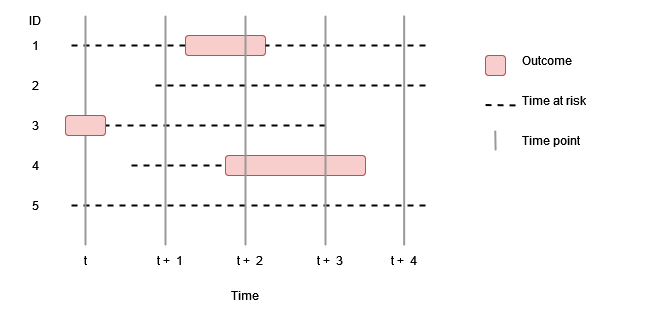
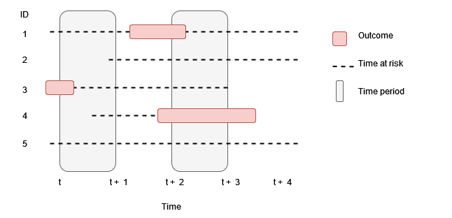
Prevalence is the total number of people with an ongoing health-related event, such as a medical condition or medication use, at a particular time or during a given period divided by the population at risk. In the previous vignettes we have seen how we can identify a denominator population and define and instantiate an outcome cohort. Prevalence then can be calculated to describe the proportion of people in the denominator population who are in the outcome cohort at a specified time point (point prevalence) or over a given time interval (period prevalence).
In the first plot below, we can We can see at time t+2 that 2 out of 5 people were in an outcome cohort, giving a point prevalence of 40%. In the second figure, period prevalence between t+2 and t+3 was also 40%. However for period prevalence between t and t+1, what do we do with those people who only contributed some time during the period? If we included them we´ll have a period prevalence of 20%, whereas if we require that everyone is observed for the full period to contribute then we´ll have a period prevalence of 33%.
Outcome definition
Outcome cohorts are defined externally. When creating outcome cohorts for estimating prevalence, important considerations relate to whether to restrict events to the first occurrence in an individuals history or not and how cohort exit is defined. These decisions will necessarily be based on the nature of the proposed outcome (e.g., whether it is an acute or chronic condition) and the research question being investigated.
In addition, it is typically not recommended to include exclusion
requirements when creating outcome cohorts. Restrictions on patient
characteristics can be specified when identifying the denominator cohort
using generateDenominatorCohortSet() or
generateTargetDenominatorCohortSet()
Using estimatePointPrevalence() and estimatePeriodPrevalence()
estimatePointPrevalence() and
estimatePeriodPrevalence() are the functions we use to
estimate prevalence. To demonstrate its use, let´s load the
IncidencePrevalence package (along with a couple of packages to help for
subsequent plots) and generate 20,000 example patients using the
mockIncidencePrevalence() function from whom we´ll create a
denominator population without adding any restrictions other than a
study period.
library(IncidencePrevalence)
library(dplyr)
library(tidyr)
library(ggplot2)
library(patchwork)

cdm <- mockIncidencePrevalence(
  sampleSize = 20000,
  earliestObservationStartDate = as.Date("1960-01-01"),
  minOutcomeDays = 365,
  outPre = 0.3
)

cdm <- generateDenominatorCohortSet(
  cdm = cdm, name = "denominator",
  cohortDateRange = c(as.Date("1990-01-01"), as.Date("2009-12-31")),
  ageGroup = list(c(0, 150)),
  sex = "Both",
  daysPriorObservation = 0
)

cdm$denominator %>%
  glimpse()
#> Rows: ??
#> Columns: 4
#> Database: DuckDB v1.3.2 [unknown@Linux 6.11.0-1018-azure:R 4.5.1/:memory:]
#> $ cohort_definition_id <int> 1, 1, 1, 1, 1, 1, 1, 1, 1, 1, 1, 1, 1, 1, 1, 1, 1…
#> $ subject_id           <int> 1, 3, 10, 12, 14, 16, 18, 19, 20, 22, 23, 25, 27,…
#> $ cohort_start_date    <date> 1991-08-05, 2007-02-16, 2009-04-21, 1992-01-28, …
#> $ cohort_end_date      <date> 1996-01-10, 2007-12-09, 2009-12-31, 1999-08-18, …
Using estimatePointPrevalence()
Let´s first calculate point prevalence on a yearly basis.
prev <- estimatePointPrevalence(
  cdm = cdm,
  denominatorTable = "denominator",
  outcomeTable = "outcome",
  interval = "Years"
)

prev %>%
  glimpse()
#> Rows: 144
#> Columns: 13
#> $ result_id        <int> 1, 1, 1, 1, 1, 1, 1, 1, 1, 1, 1, 1, 1, 1, 1, 1, 1, 1,…
#> $ cdm_name         <chr> "mock", "mock", "mock", "mock", "mock", "mock", "mock…
#> $ group_name       <chr> "denominator_cohort_name &&& outcome_cohort_name", "d…
#> $ group_level      <chr> "denominator_cohort_1 &&& cohort_1", "denominator_coh…
#> $ strata_name      <chr> "overall", "overall", "overall", "overall", "overall"…
#> $ strata_level     <chr> "overall", "overall", "overall", "overall", "overall"…
#> $ variable_name    <chr> "Denominator", "Outcome", "Outcome", "Outcome", "Outc…
#> $ variable_level   <chr> NA, NA, NA, NA, NA, NA, NA, NA, NA, NA, NA, NA, NA, N…
#> $ estimate_name    <chr> "denominator_count", "outcome_count", "prevalence", "…
#> $ estimate_type    <chr> "integer", "integer", "numeric", "numeric", "numeric"…
#> $ estimate_value   <chr> "2147", "82", "0.03819", "0.03088", "0.04716", "2164"…
#> $ additional_name  <chr> "prevalence_start_date &&& prevalence_end_date &&& an…
#> $ additional_level <chr> "1990-01-01 &&& 1990-01-01 &&& years", "1990-01-01 &&…

plotPrevalence(prev)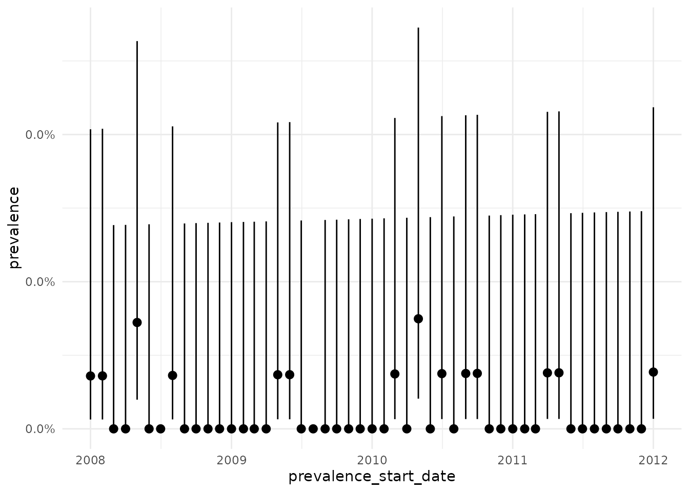
As well as plotting our prevalence estimates, we can also plot the population for whom these were calculated. Here we´ll plot outcome and population counts together.
outcome_plot <- plotPrevalencePopulation(result = prev, y = "outcome_count") + xlab("") +
  theme(axis.text.x = element_blank()) +
  ggtitle("a) Number of outcomes by year")
denominator_plot <- plotPrevalencePopulation(result = prev) +
  ggtitle("b) Number of people in denominator population by year")
outcome_plot / denominator_plot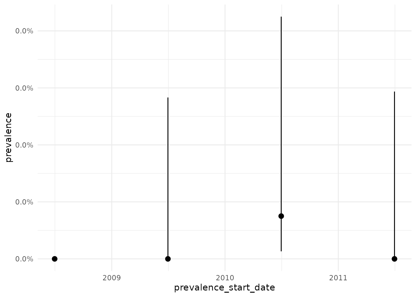
We can also calculate point prevalence by calendar month.
prev <- estimatePointPrevalence(
  cdm = cdm,
  denominatorTable = "denominator",
  outcomeTable = "outcome",
  interval = "Months"
)

prev %>%
  glimpse()
#> Rows: 1,244
#> Columns: 13
#> $ result_id        <int> 1, 1, 1, 1, 1, 1, 1, 1, 1, 1, 1, 1, 1, 1, 1, 1, 1, 1,…
#> $ cdm_name         <chr> "mock", "mock", "mock", "mock", "mock", "mock", "mock…
#> $ group_name       <chr> "denominator_cohort_name &&& outcome_cohort_name", "d…
#> $ group_level      <chr> "denominator_cohort_1 &&& cohort_1", "denominator_coh…
#> $ strata_name      <chr> "overall", "overall", "overall", "overall", "overall"…
#> $ strata_level     <chr> "overall", "overall", "overall", "overall", "overall"…
#> $ variable_name    <chr> "Denominator", "Outcome", "Outcome", "Outcome", "Outc…
#> $ variable_level   <chr> NA, NA, NA, NA, NA, NA, NA, NA, NA, NA, NA, NA, NA, N…
#> $ estimate_name    <chr> "denominator_count", "outcome_count", "prevalence", "…
#> $ estimate_type    <chr> "integer", "integer", "numeric", "numeric", "numeric"…
#> $ estimate_value   <chr> "2147", "82", "0.03819", "0.03088", "0.04716", "2148"…
#> $ additional_name  <chr> "prevalence_start_date &&& prevalence_end_date &&& an…
#> $ additional_level <chr> "1990-01-01 &&& 1990-01-01 &&& months", "1990-01-01 &…

plotPrevalence(prev)
By using the estimatePointPrevalence() function, we can further specify where to compute point prevalence in each time interval (start, middle, end). By default, this parameter is set to start. But we can use middle instead like so:
prev <- estimatePointPrevalence(
  cdm = cdm,
  denominatorTable = "denominator",
  outcomeTable = "outcome",
  interval = "Years",
  timePoint = "middle"
)

prev %>%
  glimpse()
#> Rows: 144
#> Columns: 13
#> $ result_id        <int> 1, 1, 1, 1, 1, 1, 1, 1, 1, 1, 1, 1, 1, 1, 1, 1, 1, 1,…
#> $ cdm_name         <chr> "mock", "mock", "mock", "mock", "mock", "mock", "mock…
#> $ group_name       <chr> "denominator_cohort_name &&& outcome_cohort_name", "d…
#> $ group_level      <chr> "denominator_cohort_1 &&& cohort_1", "denominator_coh…
#> $ strata_name      <chr> "overall", "overall", "overall", "overall", "overall"…
#> $ strata_level     <chr> "overall", "overall", "overall", "overall", "overall"…
#> $ variable_name    <chr> "Denominator", "Outcome", "Outcome", "Outcome", "Outc…
#> $ variable_level   <chr> NA, NA, NA, NA, NA, NA, NA, NA, NA, NA, NA, NA, NA, N…
#> $ estimate_name    <chr> "denominator_count", "outcome_count", "prevalence", "…
#> $ estimate_type    <chr> "integer", "integer", "numeric", "numeric", "numeric"…
#> $ estimate_value   <chr> "2160", "76", "0.03519", "0.0282", "0.04382", "2161",…
#> $ additional_name  <chr> "prevalence_start_date &&& prevalence_end_date &&& an…
#> $ additional_level <chr> "1990-07-01 &&& 1990-07-01 &&& years", "1990-07-01 &&…

plotPrevalence(prev, line = FALSE)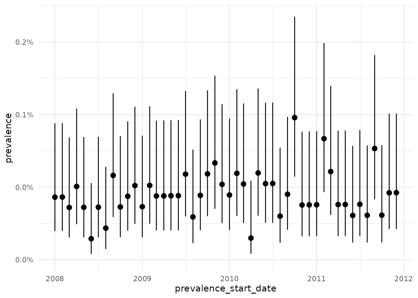
Using estimatePeriodPrevalence()
To calculate period prevalence by year (i.e. each period is a calendar year)
prev <- estimatePeriodPrevalence(
  cdm = cdm,
  denominatorTable = "denominator",
  outcomeTable = "outcome",
  interval = "Years"
)

prev %>%
  glimpse()
#> Rows: 144
#> Columns: 13
#> $ result_id        <int> 1, 1, 1, 1, 1, 1, 1, 1, 1, 1, 1, 1, 1, 1, 1, 1, 1, 1,…
#> $ cdm_name         <chr> "mock", "mock", "mock", "mock", "mock", "mock", "mock…
#> $ group_name       <chr> "denominator_cohort_name &&& outcome_cohort_name", "d…
#> $ group_level      <chr> "denominator_cohort_1 &&& cohort_1", "denominator_coh…
#> $ strata_name      <chr> "overall", "overall", "overall", "overall", "overall"…
#> $ strata_level     <chr> "overall", "overall", "overall", "overall", "overall"…
#> $ variable_name    <chr> "Denominator", "Outcome", "Outcome", "Outcome", "Outc…
#> $ variable_level   <chr> NA, NA, NA, NA, NA, NA, NA, NA, NA, NA, NA, NA, NA, N…
#> $ estimate_name    <chr> "denominator_count", "outcome_count", "prevalence", "…
#> $ estimate_type    <chr> "integer", "integer", "numeric", "numeric", "numeric"…
#> $ estimate_value   <chr> "2523", "189", "0.07491", "0.06527", "0.08584", "2517…
#> $ additional_name  <chr> "prevalence_start_date &&& prevalence_end_date &&& an…
#> $ additional_level <chr> "1990-01-01 &&& 1990-12-31 &&& years", "1990-01-01 &&…

plotPrevalence(prev)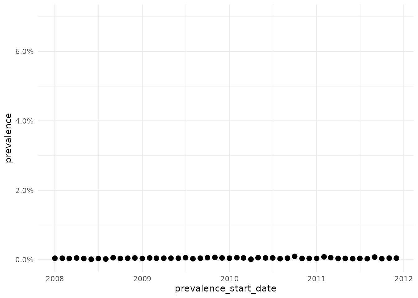
To calculate period prevalence by month (i.e. each period is a calendar month)
prev <- estimatePeriodPrevalence(
  cdm = cdm,
  denominatorTable = "denominator",
  outcomeTable = "outcome",
  interval = "Months"
)

prev %>%
  glimpse()
#> Rows: 1,244
#> Columns: 13
#> $ result_id        <int> 1, 1, 1, 1, 1, 1, 1, 1, 1, 1, 1, 1, 1, 1, 1, 1, 1, 1,…
#> $ cdm_name         <chr> "mock", "mock", "mock", "mock", "mock", "mock", "mock…
#> $ group_name       <chr> "denominator_cohort_name &&& outcome_cohort_name", "d…
#> $ group_level      <chr> "denominator_cohort_1 &&& cohort_1", "denominator_coh…
#> $ strata_name      <chr> "overall", "overall", "overall", "overall", "overall"…
#> $ strata_level     <chr> "overall", "overall", "overall", "overall", "overall"…
#> $ variable_name    <chr> "Denominator", "Outcome", "Outcome", "Outcome", "Outc…
#> $ variable_level   <chr> NA, NA, NA, NA, NA, NA, NA, NA, NA, NA, NA, NA, NA, N…
#> $ estimate_name    <chr> "denominator_count", "outcome_count", "prevalence", "…
#> $ estimate_type    <chr> "integer", "integer", "numeric", "numeric", "numeric"…
#> $ estimate_value   <chr> "2176", "94", "0.0432", "0.03543", "0.05258", "2171",…
#> $ additional_name  <chr> "prevalence_start_date &&& prevalence_end_date &&& an…
#> $ additional_level <chr> "1990-01-01 &&& 1990-01-31 &&& months", "1990-01-01 &…

plotPrevalence(prev)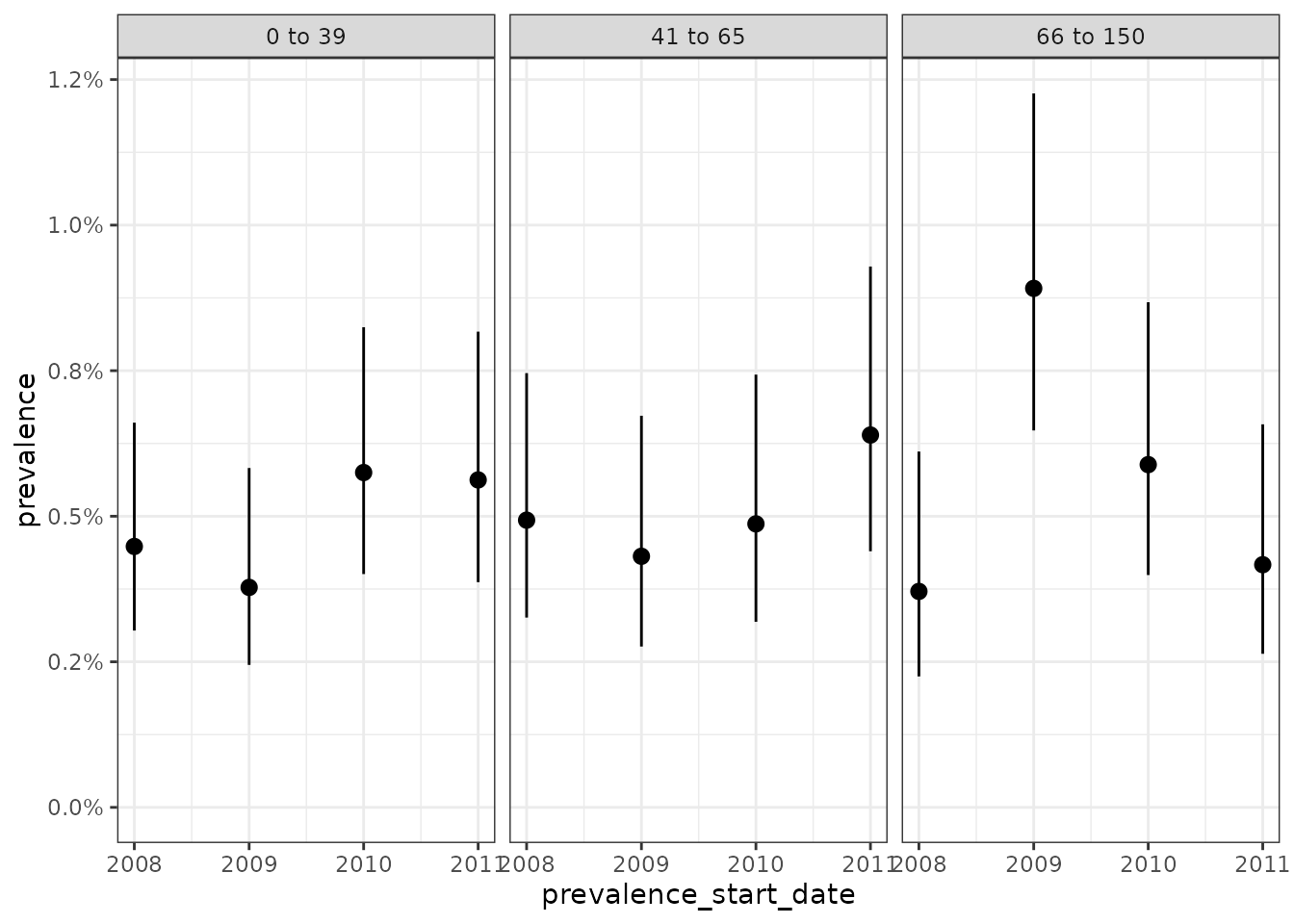
When using the estimatePeriodPrevalence() function, we can set the fullContribution parameter to decide whether individuals are required to be present in the database throughout the interval of interest in order to be included (fullContribution=TRUE). If not, individuals will only be required to be present for one day of the interval to contribute (fullContribution=FALSE), which would be specified like so:
prev <- estimatePeriodPrevalence(
  cdm = cdm,
  denominatorTable = "denominator",
  outcomeTable = "outcome",
  interval = "Months",
  fullContribution = FALSE
)

prev %>%
  glimpse()
#> Rows: 1,244
#> Columns: 13
#> $ result_id        <int> 1, 1, 1, 1, 1, 1, 1, 1, 1, 1, 1, 1, 1, 1, 1, 1, 1, 1,…
#> $ cdm_name         <chr> "mock", "mock", "mock", "mock", "mock", "mock", "mock…
#> $ group_name       <chr> "denominator_cohort_name &&& outcome_cohort_name", "d…
#> $ group_level      <chr> "denominator_cohort_1 &&& cohort_1", "denominator_coh…
#> $ strata_name      <chr> "overall", "overall", "overall", "overall", "overall"…
#> $ strata_level     <chr> "overall", "overall", "overall", "overall", "overall"…
#> $ variable_name    <chr> "Denominator", "Outcome", "Outcome", "Outcome", "Outc…
#> $ variable_level   <chr> NA, NA, NA, NA, NA, NA, NA, NA, NA, NA, NA, NA, NA, N…
#> $ estimate_name    <chr> "denominator_count", "outcome_count", "prevalence", "…
#> $ estimate_type    <chr> "integer", "integer", "numeric", "numeric", "numeric"…
#> $ estimate_value   <chr> "2176", "94", "0.0432", "0.03543", "0.05258", "2171",…
#> $ additional_name  <chr> "prevalence_start_date &&& prevalence_end_date &&& an…
#> $ additional_level <chr> "1990-01-01 &&& 1990-01-31 &&& months", "1990-01-01 &…

plotPrevalence(prev)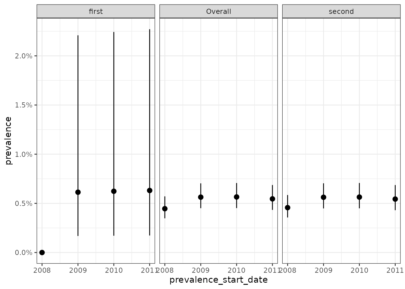
Stratified analyses
If we specified multiple denominator populations results will be returned for each. Here for example we define three age groups for denominator populations and get three sets of estimates back when estimating prevalence.
cdm <- generateDenominatorCohortSet(
  cdm = cdm, name = "denominator_age_sex",
  cohortDateRange = c(as.Date("1990-01-01"), as.Date("2009-12-31")),
  ageGroup = list(
    c(0, 39),
    c(41, 65),
    c(66, 150)
  ),
  sex = "Both",
  daysPriorObservation = 0
)
prev <- estimatePeriodPrevalence(
  cdm = cdm,
  denominatorTable = "denominator_age_sex",
  outcomeTable = "outcome"
)

plotPrevalence(prev) +
  facet_wrap(vars(denominator_age_group), ncol = 1)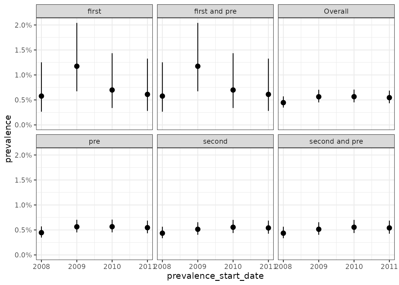
We can also plot a count of the denominator by year for each strata.
denominator_plot <- plotPrevalencePopulation(result = prev)

denominator_plot +
  facet_wrap(vars(denominator_age_group), ncol = 1)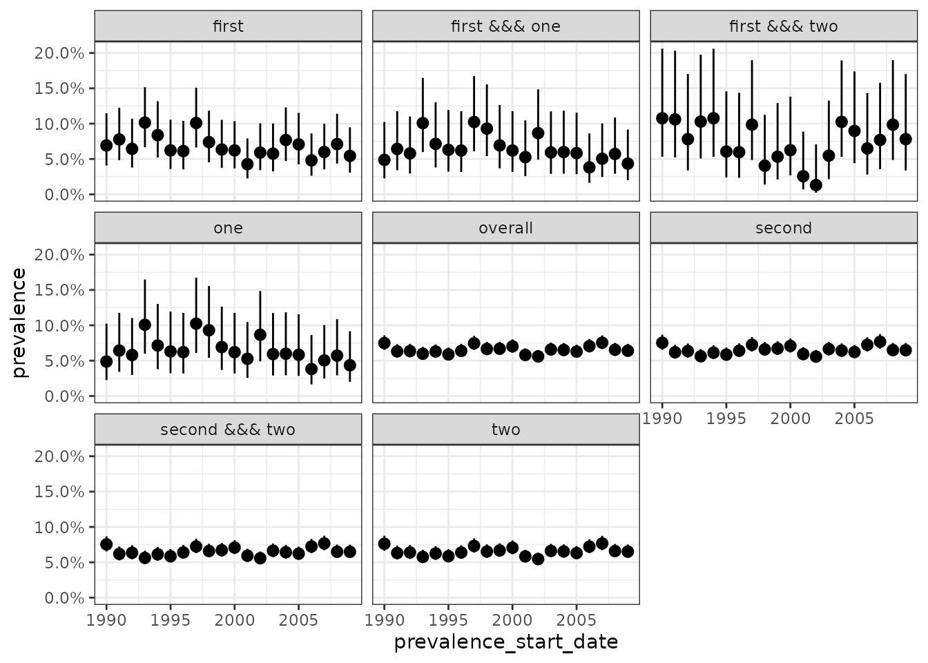
While we specify time-varying stratifications when defining our denominator populations, if we have time-invariant stratifications we can include these at the the estimation stage. To do this we first need to add a new column to our denominator cohort with our stratification variable. Here we’ll add an example stratification just to show the idea. Note, as well as getting stratified results we’ll also get overall results.
cdm$denominator <- cdm$denominator %>%
  mutate(group = if_else(as.numeric(subject_id) < 500, "first", "second"))

prev <- estimatePeriodPrevalence(
  cdm = cdm,
  denominatorTable = "denominator",
  outcomeTable = "outcome",
  strata = "group"
)

plotPrevalence(prev,
  colour = "group"
) +
  facet_wrap(vars(group), ncol = 1)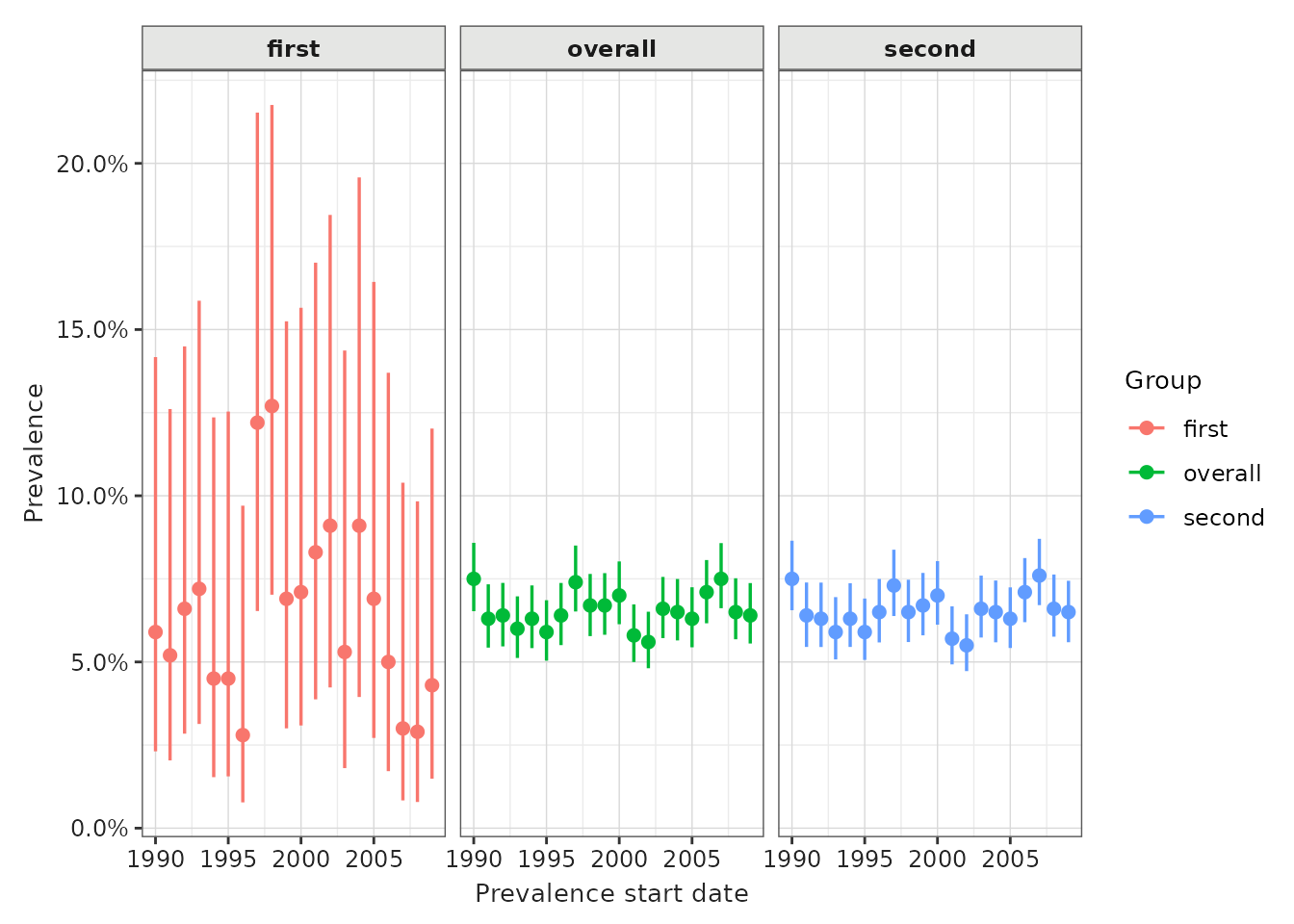
We can also stratify on multiple variables at the same time.
cdm$denominator <- cdm$denominator %>%
  mutate(
    group_1 = if_else(as.numeric(subject_id) < 1500, "first", "second"),
    group_2 = if_else(as.numeric(subject_id) < 1000, "one", "two")
  )

prev <- estimatePeriodPrevalence(
  cdm = cdm,
  denominatorTable = "denominator",
  outcomeTable = "outcome",
  strata = list(
    c("group_1"), # for just group_1
    c("group_2"), # for just group_2
    c("group_1", "group_2")
  ) # for group_1 and group_2
)

plotPrevalence(prev) +
  facet_wrap(vars(group_1, group_2), ncol = 2)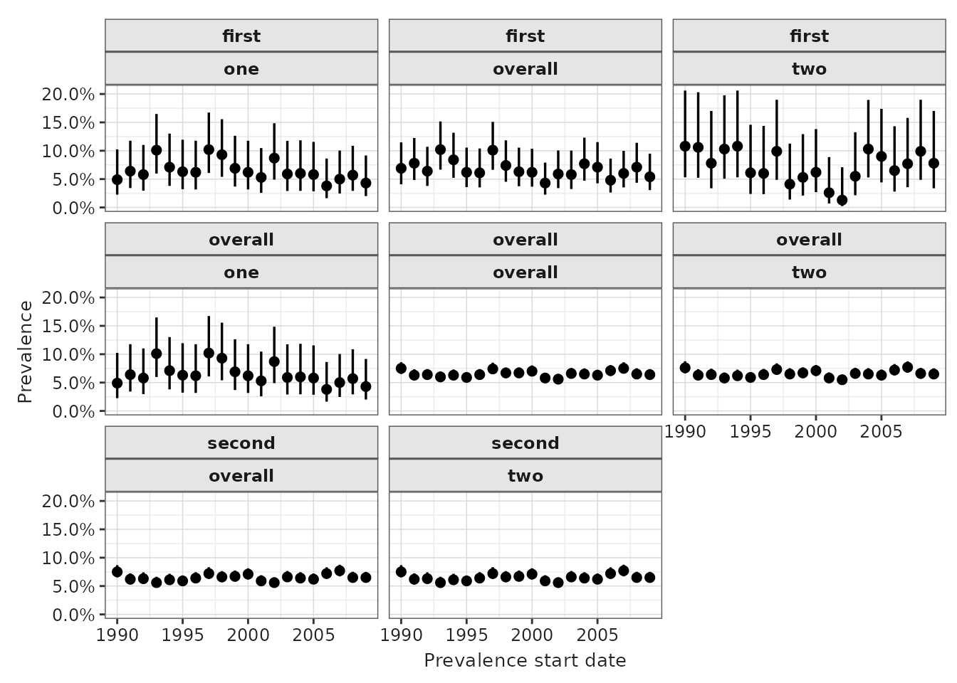
Other parameters
In the examples above, we have used calculated prevalence by months and years, but it can be also calculated by weeks, months or for the entire time period observed (overall). In addition, the user can decide whether to include time intervals that are not fully captured in the database (e.g., having data up to June for the last study year when computing period prevalence rates). By default, incidence will only be estimated for those intervals where the database captures all the interval (completeDatabaseIntervals=TRUE).
Given that we can set estimatePointPrevalence() and
estimatePeriorPrevalence() to exclude individuals based on
certain parameters (e.g., fullContribution), it is important to note
that the denominator population used to compute prevalence rates might
differ from the one calculated with
generateDenominatorCohortSet(). Along with our central
estimate, 95 % confidence intervals are calculated using the Wilson
Score method.
Attrition
estimatePointPrevalence() and
estimatePeriorPrevalence() will generate a table with point
and period prevalence rates for each of the time intervals studied and
for each combination of the parameters set, respectively. We can also
view attrition associated with performing the analysis.
prev <- estimatePeriodPrevalence(
  cdm = cdm,
  denominatorTable = "denominator",
  outcomeTable = "outcome",
  interval = "Years",
  fullContribution = TRUE
)
tablePrevalenceAttrition(prev, style = "darwin")| Reason |
Variable name
|
|||
|---|---|---|---|---|
| Number records | Number subjects | Excluded records | Excluded subjects | |
| mock; cohort_1 | ||||
| Starting population | 20,000 | 20,000 | - | - |
| Missing year of birth | 20,000 | 20,000 | 0 | 0 |
| Missing sex | 20,000 | 20,000 | 0 | 0 |
| Cannot satisfy age criteria during the study period based on year of birth | 20,000 | 20,000 | 0 | 0 |
| No observation time available during study period | 10,399 | 10,399 | 9,601 | 9,601 |
| Doesn't satisfy age criteria during the study period | 10,399 | 10,399 | 0 | 0 |
| Prior history requirement not fulfilled during study period | 10,399 | 10,399 | 0 | 0 |
| No observation time available after applying age, prior observation and, if applicable, target criteria | 10,149 | 10,149 | 250 | 250 |
| Starting analysis population | 10,149 | 10,149 | - | - |
| Not observed during the complete database interval | 10,149 | 10,149 | 0 | 0 |
| Do not satisfy full contribution requirement for an interval | 8,385 | 8,385 | 1,764 | 1,764 |