
Creating denominator cohorts
Source:vignettes/a02_Creating_denominator_populations.Rmd
a02_Creating_denominator_populations.RmdIntroduction
Calculating incidence or prevalence requires first identifying an
appropriate denominator population. To find such a denominator
population (or multiple denominator populations) we can use the
generateDenominatorCohortSet() function. This function will
identify the time that people in the database satisfy a set of criteria
related to the study period and individuals´ age, sex, and amount of
prior observed history.
When using generateDenominatorCohortSet() individuals
will enter a denominator population on the respective date of the latest
of the following:
- Study start date
- Date at which they have sufficient prior observation
- Date at which they reach a minimum age
They will then exit on the respective date of the earliest of the following:
- Study end date
- Date at which their observation period ends
- The last day in which they have the maximum age
Let´s go through a few examples to make this logic a little more concrete.
No specific requirements
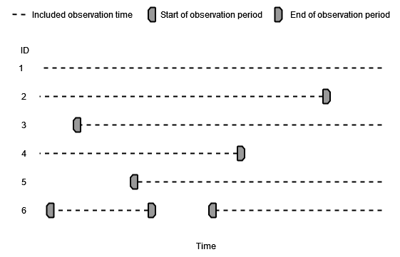
The simplest case is that no study start and end dates are specified, no prior history requirement is imposed, nor any age or sex criteria. In this case individuals will enter the denominator population once they have entered the database (start of observation period) and will leave when they exit the database (end of observation period). Note that in some databases a person can have multiple observation periods, in which case their contribution of person time would look like the the last person below.
Specified study period
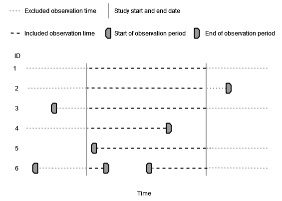
If we specify a study start and end date then only observation time during this period will be included.
Specified study period and prior history requirement
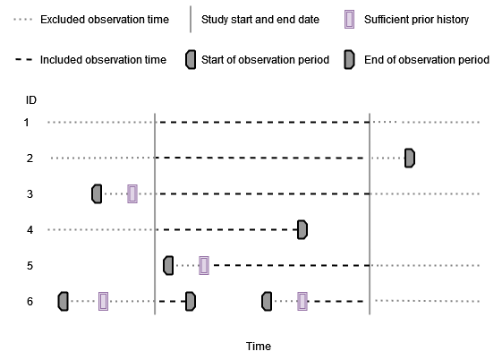
If we also add some requirement of prior history then somebody will only contribute time at risk once this is reached.
Specified study period, prior history requirement, and age and sex criteria
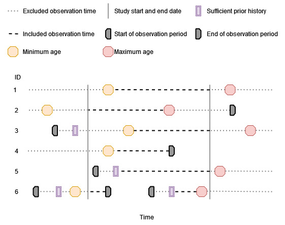
Lastly we can also impose age and sex criteria, and now individuals will only contribute time when they also satisfy these criteria. Not shown in the below figure is a person´s sex, but we could also stratify a denominator population by this as well.
Using generateDenominatorCohortSet()
generateDenominatorCohortSet() is the function we use to
identify a set of denominator populations. To demonstrate its use, let´s
load the IncidencePrevalence package (along with a couple of packages to
help for subsequent plots) and generate 500 example patients using the
mockIncidencePrevalence() function.
cdm <- mockIncidencePrevalence(sampleSize = 500)No specific requirements
We can get a denominator population without including any particular requirements like so
cdm <- generateDenominatorCohortSet(
  cdm = cdm,
  name = "denominator",
  cohortDateRange = as.Date(c(NA, NA)),
  ageGroup = list(c(0, 150)),
  sex = "Both",
  daysPriorObservation = 0
)
cdm$denominator
#> # Source:   table<denominator> [?? x 4]
#> # Database: DuckDB v1.3.2 [unknown@Linux 6.11.0-1018-azure:R 4.5.1/:memory:]
#>    cohort_definition_id subject_id cohort_start_date cohort_end_date
#>                   <int>      <int> <date>            <date>
#>  1                    1          4 1974-04-03        1982-01-16
#>  2                    1          6 1990-10-30        1996-06-28
#>  3                    1          7 1995-10-09        1997-02-28
#>  4                    1          9 1984-04-14        1989-04-07
#>  5                    1         11 2004-04-10        2012-09-24
#>  6                    1         12 2004-11-14        2007-04-29
#>  7                    1         13 2000-06-29        2004-06-13
#>  8                    1         15 1995-03-27        2005-09-01
#>  9                    1         16 2009-02-24        2011-09-29
#> 10                    1         17 2003-04-03        2006-01-26
#> # ℹ more rows

cdm$denominator %>%
  filter(subject_id %in% c("1", "2", "3", "4", "5"))
#> # Source:   SQL [?? x 4]
#> # Database: DuckDB v1.3.2 [unknown@Linux 6.11.0-1018-azure:R 4.5.1/:memory:]
#>   cohort_definition_id subject_id cohort_start_date cohort_end_date
#>                  <int>      <int> <date>            <date>
#> 1                    1          4 1974-04-03        1982-01-16
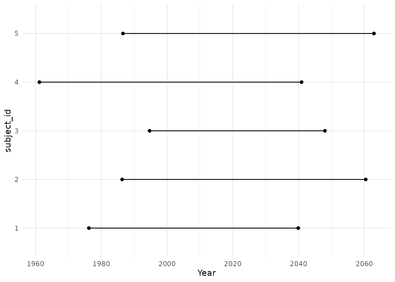
Let´s have a look at the included time of the first five patients. We can see that people enter and leave at different times.
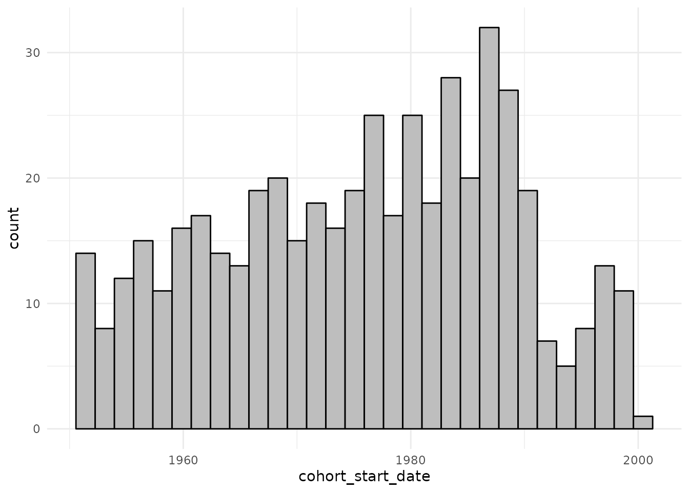
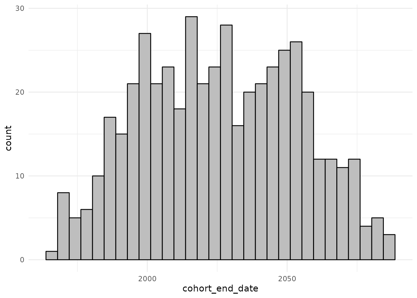
We can also plot a histogram of start and end dates of the 500 simulated patients
cdm$denominator %>%
  collect() %>%
  ggplot() +
  theme_minimal() +
  geom_histogram(aes(cohort_start_date),
    colour = "black", fill = "grey"
  )
cdm$denominator %>%
  collect() %>%
  ggplot() +
  theme_minimal() +
  geom_histogram(aes(cohort_end_date),
    colour = "black", fill = "grey"
  )
Specified study period
We can get specify a study period like so
cdm <- generateDenominatorCohortSet(
  cdm = cdm,
  name = "denominator",
  cohortDateRange = c(as.Date("1990-01-01"), as.Date("2009-12-31")),
  ageGroup = list(c(0, 150)),
  sex = "Both",
  daysPriorObservation = 0
)
cdm$denominator
#> # Source:   table<denominator> [?? x 4]
#> # Database: DuckDB v1.3.2 [unknown@Linux 6.11.0-1018-azure:R 4.5.1/:memory:]
#>    cohort_definition_id subject_id cohort_start_date cohort_end_date
#>                   <int>      <int> <date>            <date>
#>  1                    1          6 1990-10-30        1996-06-28
#>  2                    1          7 1995-10-09        1997-02-28
#>  3                    1         11 2004-04-10        2009-12-31
#>  4                    1         12 2004-11-14        2007-04-29
#>  5                    1         13 2000-06-29        2004-06-13
#>  6                    1         15 1995-03-27        2005-09-01
#>  7                    1         16 2009-02-24        2009-12-31
#>  8                    1         17 2003-04-03        2006-01-26
#>  9                    1         21 1991-11-16        2000-05-05
#> 10                    1         28 2005-11-16        2007-03-12
#> # ℹ more rows

cohortCount(cdm$denominator)
#> # A tibble: 1 × 3
#>   cohort_definition_id number_records number_subjects
#>                  <int>          <int>           <int>
#> 1                    1             97              97

cdm$denominator %>%
  filter(subject_id %in% c("1", "2", "3", "4", "5"))
#> # Source:   SQL [?? x 4]
#> # Database: DuckDB v1.3.2 [unknown@Linux 6.11.0-1018-azure:R 4.5.1/:memory:]
#> # ℹ 4 variables: cohort_definition_id <int>, subject_id <int>,
#> #   cohort_start_date <date>, cohort_end_date <date>
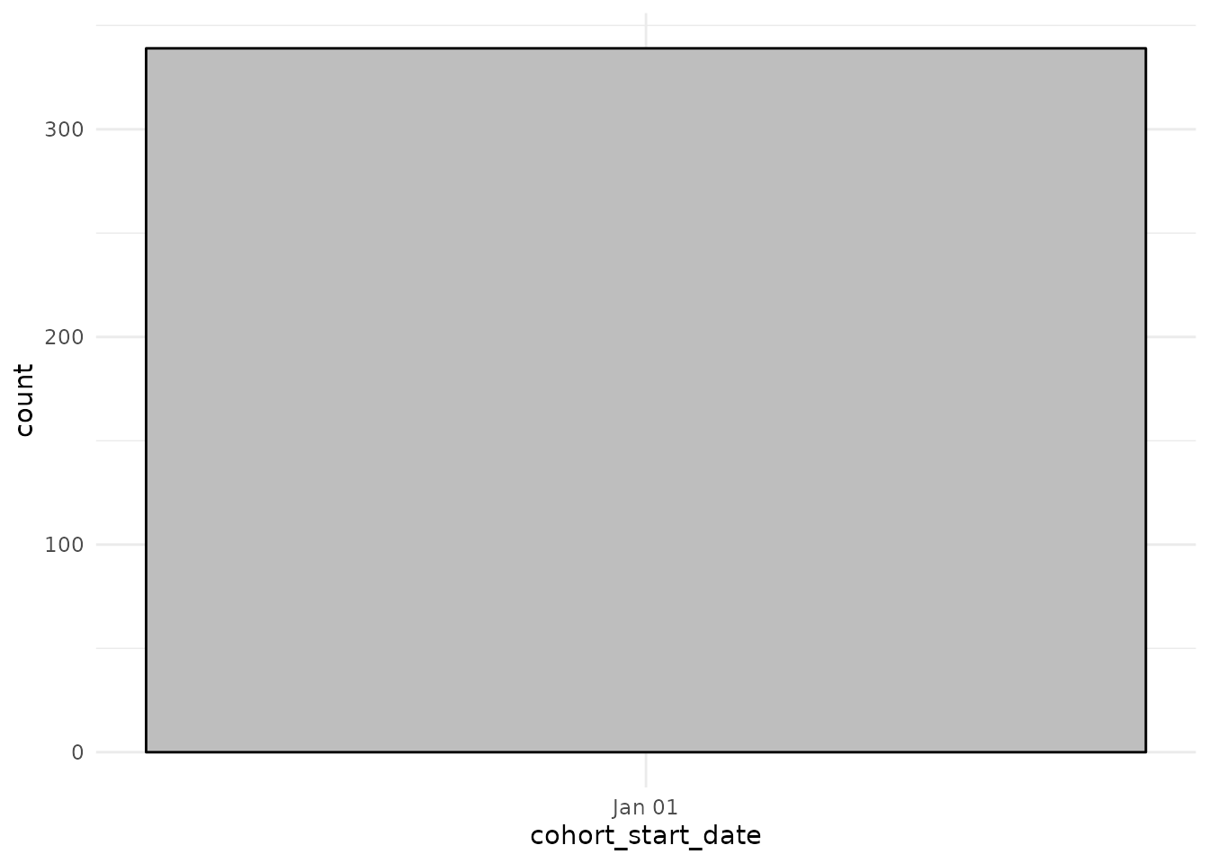
Now we can see that many more people share the same cohort entry (the study start date) and cohort exit (the study end date).
cdm$denominator %>%
  collect() %>%
  ggplot() +
  theme_minimal() +
  geom_histogram(aes(cohort_start_date),
    colour = "black", fill = "grey"
  )
cdm$denominator %>%
  collect() %>%
  ggplot() +
  theme_minimal() +
  geom_histogram(aes(cohort_end_date),
    colour = "black", fill = "grey"
  )
Specified study period and prior history requirement
We can add some requirement of prior history
cdm <- generateDenominatorCohortSet(
  cdm = cdm,
  name = "denominator",
  cohortDateRange = c(as.Date("1990-01-01"), as.Date("2009-12-31")),
  ageGroup = list(c(0, 150)),
  sex = "Both",
  daysPriorObservation = 365
)
cdm$denominator
#> # Source:   table<denominator> [?? x 4]
#> # Database: DuckDB v1.3.2 [unknown@Linux 6.11.0-1018-azure:R 4.5.1/:memory:]
#>    cohort_definition_id subject_id cohort_start_date cohort_end_date
#>                   <int>      <int> <date>            <date>
#>  1                    1          6 1991-10-30        1996-06-28
#>  2                    1          7 1996-10-08        1997-02-28
#>  3                    1         11 2005-04-10        2009-12-31
#>  4                    1         12 2005-11-14        2007-04-29
#>  5                    1         13 2001-06-29        2004-06-13
#>  6                    1         15 1996-03-26        2005-09-01
#>  7                    1         17 2004-04-02        2006-01-26
#>  8                    1         21 1992-11-15        2000-05-05
#>  9                    1         28 2006-11-16        2007-03-12
#> 10                    1         35 1990-01-01        1991-07-05
#> # ℹ more rows

cohortCount(cdm$denominator)
#> # A tibble: 1 × 3
#>   cohort_definition_id number_records number_subjects
#>                  <int>          <int>           <int>
#> 1                    1             85              85

cdm$denominator %>%
  filter(subject_id %in% c("1", "2", "3", "4", "5"))
#> # Source:   SQL [?? x 4]
#> # Database: DuckDB v1.3.2 [unknown@Linux 6.11.0-1018-azure:R 4.5.1/:memory:]
#> # ℹ 4 variables: cohort_definition_id <int>, subject_id <int>,
#> #   cohort_start_date <date>, cohort_end_date <date>
Specified study period, prior history requirement, and age and sex criteria
In addition to all the above we could also add some requirements around age and sex. One thing to note is that the age upper limit will include time from a person up to the day before their reach the age upper limit + 1 year. For instance, when the upper limit is 65, that means we will include time from a person up to and including the day before their 66th birthday.
cdm <- generateDenominatorCohortSet(
  cdm = cdm,
  name = "denominator",
  cohortDateRange = c(as.Date("1990-01-01"), as.Date("2009-12-31")),
  ageGroup = list(c(18, 65)),
  sex = "Female",
  daysPriorObservation = 365
)
cdm$denominator %>%
  glimpse()
#> Rows: ??
#> Columns: 4
#> Database: DuckDB v1.3.2 [unknown@Linux 6.11.0-1018-azure:R 4.5.1/:memory:]
#> $ cohort_definition_id <int> 1, 1, 1, 1, 1, 1, 1, 1, 1, 1, 1, 1, 1, 1, 1, 1, 1…
#> $ subject_id           <int> 6, 7, 21, 41, 62, 72, 79, 115, 122, 142, 163, 197…
#> $ cohort_start_date    <date> 1991-10-30, 1996-10-08, 1992-11-15, 1991-11-22, …
#> $ cohort_end_date      <date> 1996-06-28, 1997-02-28, 2000-05-05, 1992-10-13, …

cohortCount(cdm$denominator)
#> # A tibble: 1 × 3
#>   cohort_definition_id number_records number_subjects
#>                  <int>          <int>           <int>
#> 1                    1             27              27

cdm$denominator %>%
  filter(subject_id %in% c("1", "2", "3", "4", "5"))
#> # Source:   SQL [?? x 4]
#> # Database: DuckDB v1.3.2 [unknown@Linux 6.11.0-1018-azure:R 4.5.1/:memory:]
#> # ℹ 4 variables: cohort_definition_id <int>, subject_id <int>,
#> #   cohort_start_date <date>, cohort_end_date <date>
Multiple options to return multiple denominator populations
More than one age, sex and prior history requirements can be specified at the same time. First, we can take a look at having two age groups. We can see below that those individuals who have their 41st birthday during the study period will go from the first cohort (age_group: 0;40) to the second (age_group: 41;100) on this day.
cdm <- mockIncidencePrevalence(
  sampleSize = 500,
  earliestObservationStartDate = as.Date("2000-01-01"),
  latestObservationStartDate = as.Date("2005-01-01"),
  minDaysToObservationEnd = 10000,
  maxDaysToObservationEnd = NULL,
  earliestDateOfBirth = as.Date("1960-01-01"),
  latestDateOfBirth = as.Date("1980-01-01")
)

cdm <- generateDenominatorCohortSet(
  cdm = cdm,
  name = "denominator",
  ageGroup = list(
    c(0, 40),
    c(41, 100)
  ),
  sex = "Both",
  daysPriorObservation = 0
)
cdm$denominator %>%
  filter(subject_id %in% !!as.character(seq(1:30))) %>%
  collect() %>%
  left_join(settings(cdm$denominator),
    by = "cohort_definition_id"
  ) %>%
  pivot_longer(cols = c(
    "cohort_start_date",
    "cohort_end_date"
  )) %>%
  mutate(subject_id = factor(as.numeric(subject_id))) %>%
  ggplot(aes(x = subject_id, y = value, colour = age_group)) +
  geom_point(position = position_dodge(width = 0.5)) +
  geom_line(position = position_dodge(width = 0.5)) +
  theme_minimal() +
  theme(
    legend.position = "top",
    legend.title = element_blank()
  ) +
  ylab("Year") +
  coord_flip()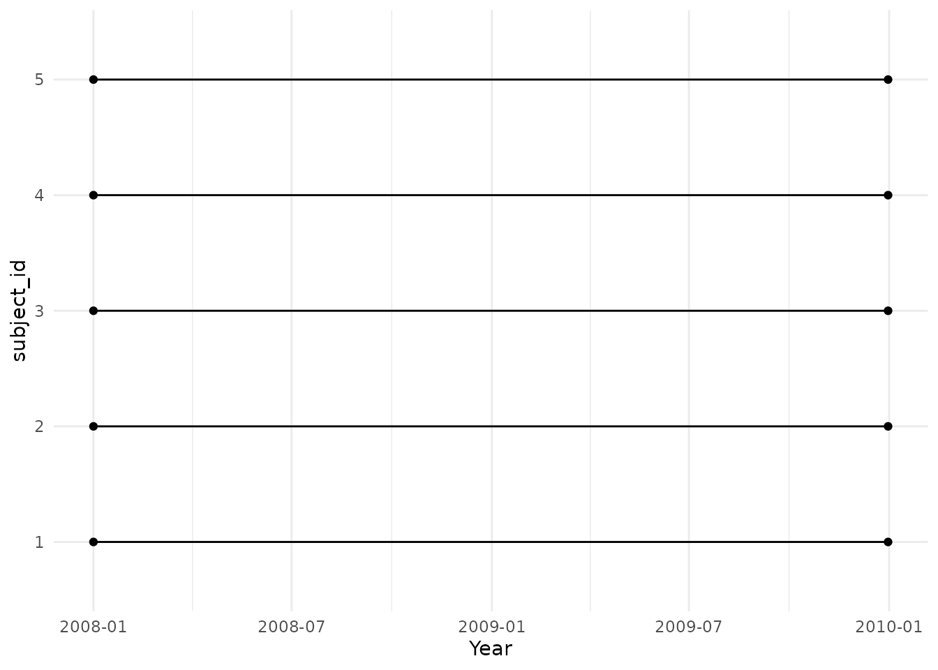
We can then also sex specific denominator cohorts.
cdm <- generateDenominatorCohortSet(
  cdm = cdm,
  name = "denominator",
  ageGroup = list(
    c(0, 40),
    c(41, 100)
  ),
  sex = c("Male", "Female", "Both"),
  daysPriorObservation = 0
)
cdm$denominator %>%
  filter(subject_id %in% !!as.character(seq(1:15))) %>%
  collect() %>%
  left_join(settings(cdm$denominator)) %>%
  pivot_longer(cols = c(
    "cohort_start_date",
    "cohort_end_date"
  )) %>%
  mutate(subject_id = factor(as.numeric(subject_id))) %>%
  ggplot(aes(x = subject_id, y = value, colour = age_group)) +
  facet_grid(sex ~ ., space = "free_y") +
  geom_point(position = position_dodge(width = 0.5)) +
  geom_line(position = position_dodge(width = 0.5)) +
  theme_bw() +
  theme(
    legend.position = "top",
    legend.title = element_blank()
  ) +
  ylab("Year") +
  coord_flip()
And we could also specifying multiple prior history requirements
cdm <- generateDenominatorCohortSet(
  cdm = cdm,
  name = "denominator",
  ageGroup = list(
    c(0, 40),
    c(41, 100)
  ),
  sex = c("Male", "Female", "Both"),
  daysPriorObservation = c(0, 365)
)
cdm$denominator %>%
  filter(subject_id %in% !!as.character(seq(1:8))) %>%
  collect() %>%
  left_join(settings(cdm$denominator)) %>%
  pivot_longer(cols = c(
    "cohort_start_date",
    "cohort_end_date"
  )) %>%
  mutate(subject_id = factor(as.numeric(subject_id))) %>%
  ggplot(aes(
    x = subject_id, y = value, colour = age_group,
    linetype = sex, shape = sex
  )) +
  facet_grid(sex + days_prior_observation ~ .,
    space = "free",
    scales = "free"
  ) +
  geom_point(position = position_dodge(width = 0.5)) +
  geom_line(position = position_dodge(width = 0.5)) +
  theme_bw() +
  theme(legend.position = "top") +
  ylab("Year") +
  coord_flip()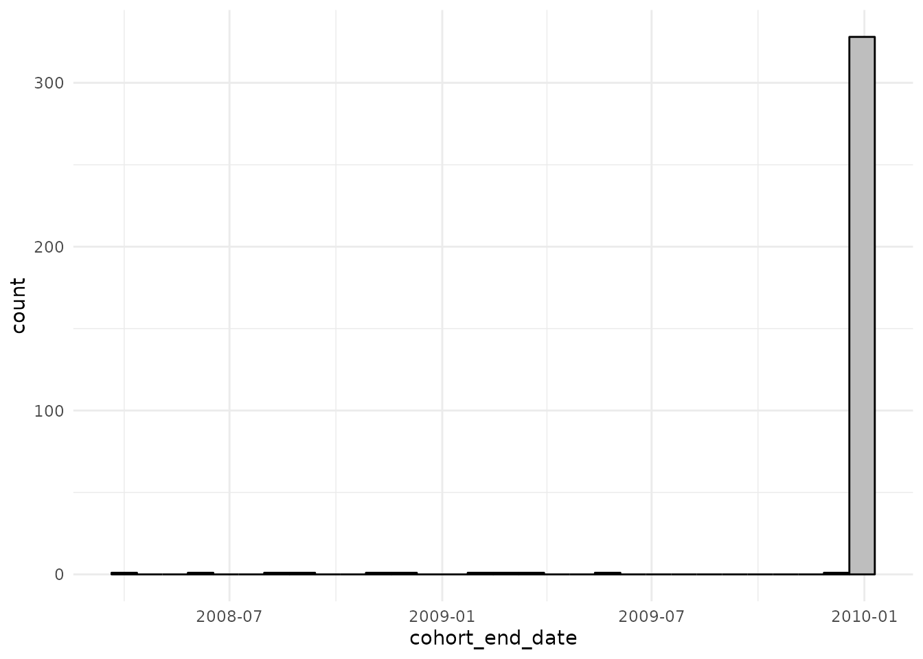
Note, setting requirementInteractions to FALSE would mean that only the first value of other age, sex, and prior history requirements are considered for a given characteristic. In this case the order of the values will be important and generally the first values will be the primary analysis settings while subsequent values are for secondary analyses.
cdm <- generateDenominatorCohortSet(
  cdm = cdm,
  name = "denominator",
  ageGroup = list(
    c(0, 40),
    c(41, 100)
  ),
  sex = c("Male", "Female", "Both"),
  daysPriorObservation = c(0, 365),
  requirementInteractions = FALSE
)

cdm$denominator %>%
  filter(subject_id %in% !!as.character(seq(1:8))) %>%
  collect() %>%
  left_join(settings(cdm$denominator)) %>%
  pivot_longer(cols = c(
    "cohort_start_date",
    "cohort_end_date"
  )) %>%
  mutate(subject_id = factor(as.numeric(subject_id))) %>%
  ggplot(aes(
    x = subject_id, y = value, colour = age_group,
    linetype = sex, shape = sex
  )) +
  facet_grid(sex + days_prior_observation ~ .,
    space = "free",
    scales = "free"
  ) +
  geom_point(position = position_dodge(width = 0.5)) +
  geom_line(position = position_dodge(width = 0.5)) +
  theme_bw() +
  theme(legend.position = "top") +
  ylab("Year") +
  coord_flip()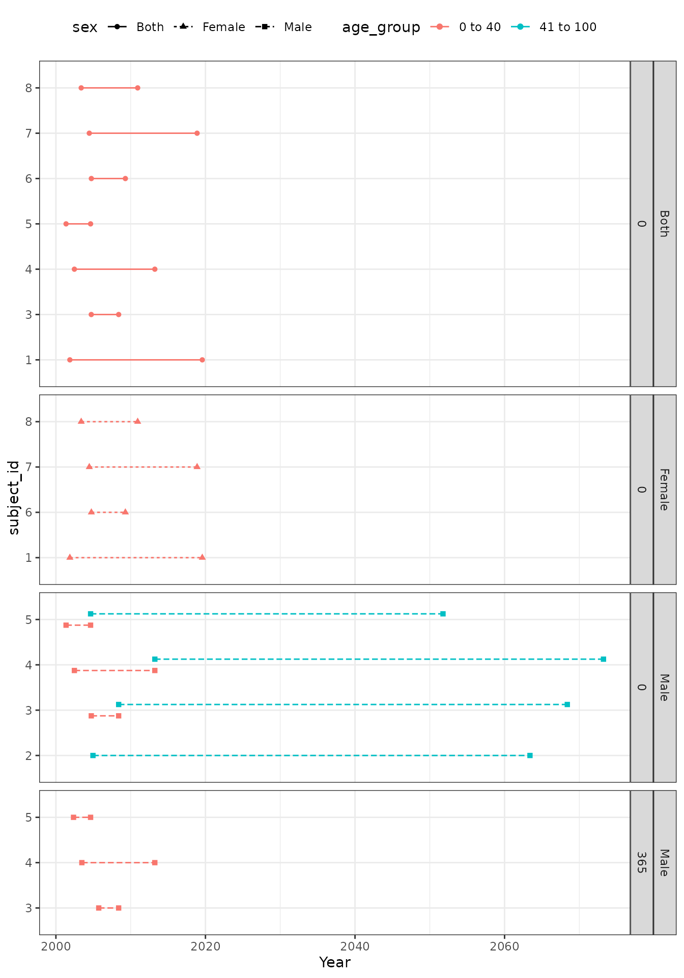
Output
generateDenominatorCohortSet() will generate a table
with the denominator population, which includes the information on all
the individuals who fulfill the given criteria at any point during the
study period. It also includes information on the specific start and end
dates in which individuals contributed to the denominator population
(cohort_start_date and cohort_end_date). Each patient is recorded in a
different row. For those databases that allow individuals to have
multiple non-overlapping observation periods, one row for each patient
and observation period is considered.
Considering the following example, we can see:
cdm <- generateDenominatorCohortSet(
  cdm = cdm,
  name = "denominator",
  cohortDateRange = c(as.Date("1990-01-01"), as.Date("2009-12-31")),
  ageGroup = list(
    c(0, 18),
    c(19, 100)
  ),
  sex = c("Male", "Female"),
  daysPriorObservation = c(0, 365)
)

head(cdm$denominator, 8)
#> # Source:   SQL [?? x 4]
#> # Database: DuckDB v1.3.2 [unknown@Linux 6.11.0-1018-azure:R 4.5.1/:memory:]
#>   cohort_definition_id subject_id cohort_start_date cohort_end_date
#>                  <int>      <int> <date>            <date>
#> 1                    5          2 2004-12-15        2009-12-31
#> 2                    5          3 2004-09-24        2009-12-31
#> 3                    5          4 2002-06-22        2009-12-31
#> 4                    5          5 2001-05-11        2009-12-31
#> 5                    5          9 2004-02-27        2009-12-31
#> 6                    5         10 2000-01-18        2009-12-31
#> 7                    5         12 2004-10-21        2009-12-31
#> 8                    5         13 2000-06-29        2009-12-31
The output table will have several attributes. With
settings() we can see the options used when defining the
set of denominator populations. More than one age, sex and prior history
requirements can be specified at the same time and each combination of
these variables will result in a different cohort, each of which has a
corresponding cohort_definition_id. In the above example, we identified
8 different cohorts:
settings(cdm$denominator) %>%
  glimpse()
#> Rows: 8
#> Columns: 11
#> $ cohort_definition_id        <int> 1, 2, 3, 4, 5, 6, 7, 8
#> $ cohort_name                 <chr> "denominator_cohort_1", "denominator_cohor…
#> $ age_group                   <chr> "0 to 18", "0 to 18", "0 to 18", "0 to 18"…
#> $ sex                         <chr> "Male", "Male", "Female", "Female", "Male"…
#> $ days_prior_observation      <dbl> 0, 365, 0, 365, 0, 365, 0, 365
#> $ start_date                  <date> 1990-01-01, 1990-01-01, 1990-01-01, 1990-0…
#> $ end_date                    <date> 2009-12-31, 2009-12-31, 2009-12-31, 2009-1…
#> $ requirements_at_entry       <chr> "FALSE", "FALSE", "FALSE", "FALSE", "FALS…
#> $ target_cohort_definition_id <int> NA, NA, NA, NA, NA, NA, NA, NA
#> $ target_cohort_name          <chr> "None", "None", "None", "None", "None", "…
#> $ time_at_risk                <chr> "0 to Inf", "0 to Inf", "0 to Inf", "0 to …
With cohortCount() we can see the number of individuals
who entered each study cohort
cohortCount(cdm$denominator) %>%
  glimpse()
#> Rows: 8
#> Columns: 3
#> $ cohort_definition_id <int> 1, 2, 3, 4, 5, 6, 7, 8
#> $ number_records       <int> 0, 0, 0, 0, 233, 233, 267, 267
#> $ number_subjects      <int> 0, 0, 0, 0, 233, 233, 267, 267
With attrition() we can see the number of individuals in
the database who were excluded from entering a given denominator
population along with the reason (such as missing crucial information or
not satisfying the sex or age criteria required, among others):
attrition(cdm$denominator) %>%
  glimpse()
#> Rows: 72
#> Columns: 7
#> $ cohort_definition_id <int> 1, 1, 1, 1, 1, 1, 1, 1, 1, 2, 2, 2, 2, 2, 2, 2, 2…
#> $ number_records       <int> 500, 500, 500, 500, 500, 500, 500, 233, 0, 500, 5…
#> $ number_subjects      <int> 500, 500, 500, 500, 500, 500, 500, 233, 0, 500, 5…
#> $ reason_id            <int> 1, 2, 3, 4, 5, 6, 7, 8, 10, 1, 2, 3, 4, 5, 6, 7, …
#> $ reason               <chr> "Starting population", "Missing year of birth", "…
#> $ excluded_records     <int> NA, 0, 0, 0, 0, 0, 0, 267, 233, NA, 0, 0, 0, 0, 0…
#> $ excluded_subjects    <int> NA, 0, 0, 0, 0, 0, 0, 267, 233, NA, 0, 0, 0, 0, 0…