Introduction to IncidencePrevalence • IncidencePrevalence

To do a study of incidence and prevalence, the analytics functions from this package that you would interact with are

generateDenominatorCohortSet() and generateTargetDenominatorCohortSet() - these function will identify a set of denominator populations from the database population as a whole, the former, or based on individuals in a target cohort, the latter
estimatePointPrevalence() and estimatePeriodPrevalence() - these function will estimate point and period prevalence for outcomes among denominator populations
estimateIncidence() - this function will estimate incidence rates for outcomes among denominator populations

Below, we show an example analysis to provide an broad overview of how this functionality provided by the IncidencePrevalence package can be used. More context and further examples for each of these functions are provided in later vignettes.

First, let’s load relevant libraries.

library(CDMConnector)
library(IncidencePrevalence)
library(dplyr)
library(tidyr)
library(ggplot2)

The IncidencePrevalence package works with data mapped to the OMOP CDM and we will first need to connect to a database, after which we can use the CDMConnector package to represent our mapped data as a cdm reference. For this example though we´ll use a synthetic cdm reference containing 50,000 hypothetical patients which we create using the mockIncidencePrevalence() function.

cdm <- mockIncidencePrevalence(
  sampleSize = 50000,
  outPre = 0.2
)

This example data already includes an outcome cohort.

cdm$outcome %>% 
  glimpse()

Once we have a cdm reference, we can use the generateDenominatorCohortSet() to identify a denominator cohort to use later when calculating incidence and prevalence. In this case we identify three denominator cohorts one with males, one with females, and one with both males and females included. For each of these cohorts only those aged between 18 and 65 from 2008 to 2012, and who had 365 days of prior history available are included.

cdm <- generateDenominatorCohortSet(
  cdm = cdm,
  name = "denominator",
  cohortDateRange = c(as.Date("2008-01-01"), as.Date("2012-01-01")),
  ageGroup = list(c(18, 65)),
  sex = c("Male", "Female", "Both"),
  daysPriorObservation = 365
)

We can see that each of our denominator cohorts is in the format of an OMOP CDM cohort:

cdm$denominator %>%
  glimpse()
#> Rows: ??
#> Columns: 4
#> Database: DuckDB v1.1.3-dev165 [unknown@Linux 6.5.0-1025-azure:R 4.4.2/:memory:]
#> $ cohort_definition_id <int> 1, 1, 1, 1, 1, 1, 1, 1, 1, 1, 1, 1, 1, 1, 1, 1, 1…
#> $ subject_id           <int> 59, 89, 126, 136, 156, 200, 208, 261, 501, 533, 5…
#> $ cohort_start_date    <date> 2008-06-24, 2008-01-01, 2008-01-01, 2008-01-01, …
#> $ cohort_end_date      <date> 2012-01-01, 2009-08-06, 2010-05-29, 2010-02-18, …

We can also see the settings associated with each cohort:

settings(cdm$denominator)
#> # A tibble: 3 × 10
#>   cohort_definition_id cohort_name        age_group sex   days_prior_observation
#>                  <int> <chr>              <chr>     <chr>                  <dbl>
#> 1                    1 denominator_cohor… 18 to 65  Male                     365
#> 2                    2 denominator_cohor… 18 to 65  Fema…                    365
#> 3                    3 denominator_cohor… 18 to 65  Both                     365
#> # ℹ 5 more variables: start_date <date>, end_date <date>,
#> #   target_cohort_definition_id <int>, target_cohort_name <chr>,
#> #   time_at_risk <chr>

And we can also see the count for each cohort

cohortCount(cdm$denominator)
#> # A tibble: 3 × 3
#>   cohort_definition_id number_records number_subjects
#>                  <int>          <int>           <int>
#> 1                    1           1128            1128
#> 2                    2           1056            1056
#> 3                    3           2184            2184

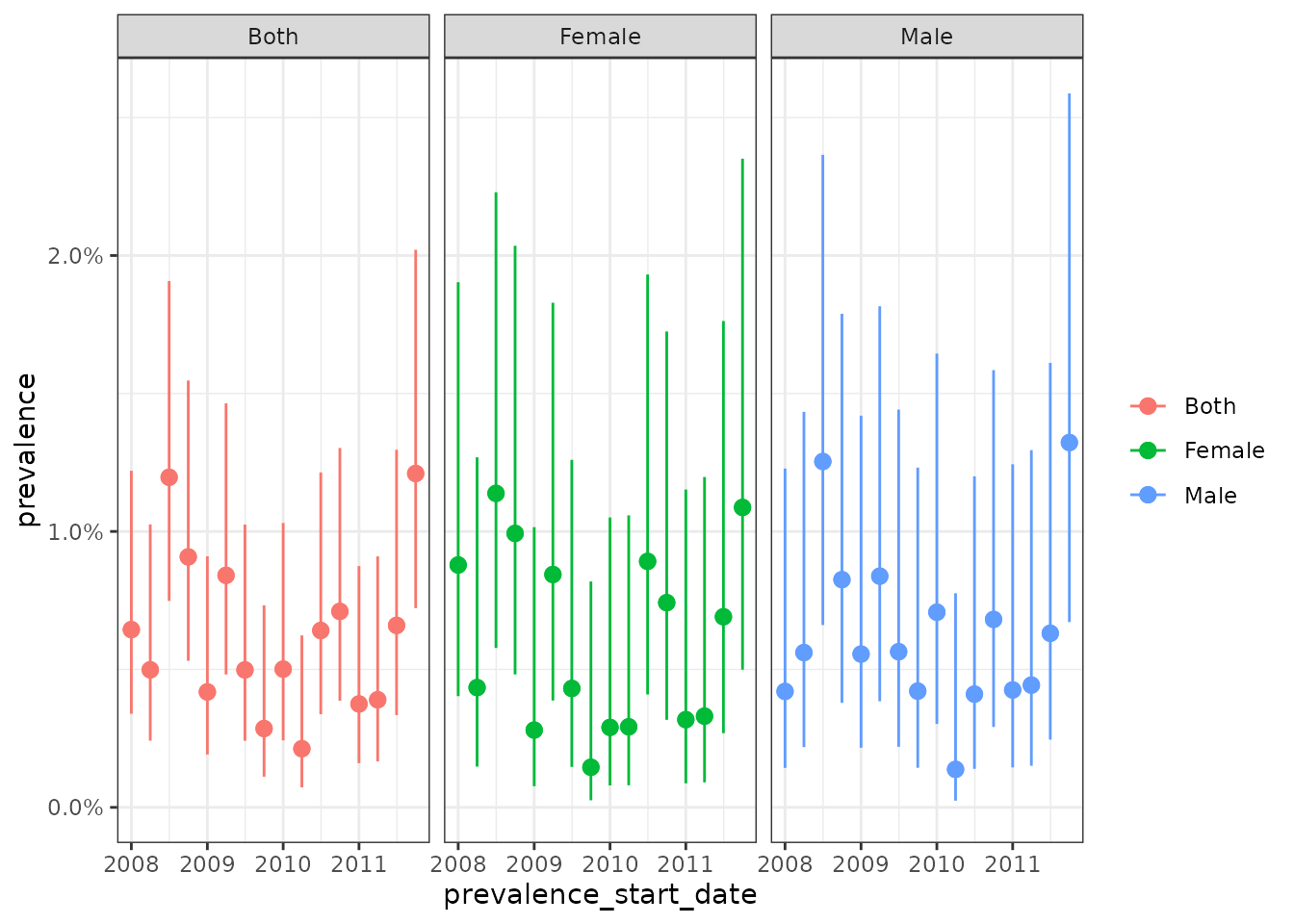
Now that we have our denominator cohorts, and using the outcome cohort that was also generated by the mockIncidencePrevalence() function, we can estimate prevalence for each using the estimatePointPrevalence() function. Here we calculate point prevalence on a yearly basis.

prev <- estimatePeriodPrevalence(
  cdm = cdm,
  denominatorTable = "denominator",
  outcomeTable = "outcome",
  interval = "quarters"
)

prev %>%
  glimpse()
#> Rows: 380
#> Columns: 13
#> $ result_id        <int> 1, 1, 1, 1, 1, 1, 1, 1, 1, 1, 1, 1, 1, 1, 1, 1, 1, 1,…
#> $ cdm_name         <chr> "mock", "mock", "mock", "mock", "mock", "mock", "mock…
#> $ group_name       <chr> "denominator_cohort_name &&& outcome_cohort_name", "d…
#> $ group_level      <chr> "denominator_cohort_3 &&& cohort_1", "denominator_coh…
#> $ strata_name      <chr> "overall", "overall", "overall", "overall", "overall"…
#> $ strata_level     <chr> "overall", "overall", "overall", "overall", "overall"…
#> $ variable_name    <chr> "Denominator", "Outcome", "Outcome", "Outcome", "Outc…
#> $ variable_level   <chr> NA, NA, NA, NA, NA, NA, NA, NA, NA, NA, NA, NA, NA, N…
#> $ estimate_name    <chr> "denominator_count", "outcome_count", "prevalence", "…
#> $ estimate_type    <chr> "integer", "integer", "numeric", "numeric", "numeric"…
#> $ estimate_value   <chr> "1397", "9", "0.00644237652111668", "0.00339303524545…
#> $ additional_name  <chr> "prevalence_start_date &&& prevalence_end_date", "pre…
#> $ additional_level <chr> "2008-01-01 &&& 2008-03-31", "2008-01-01 &&& 2008-03-…

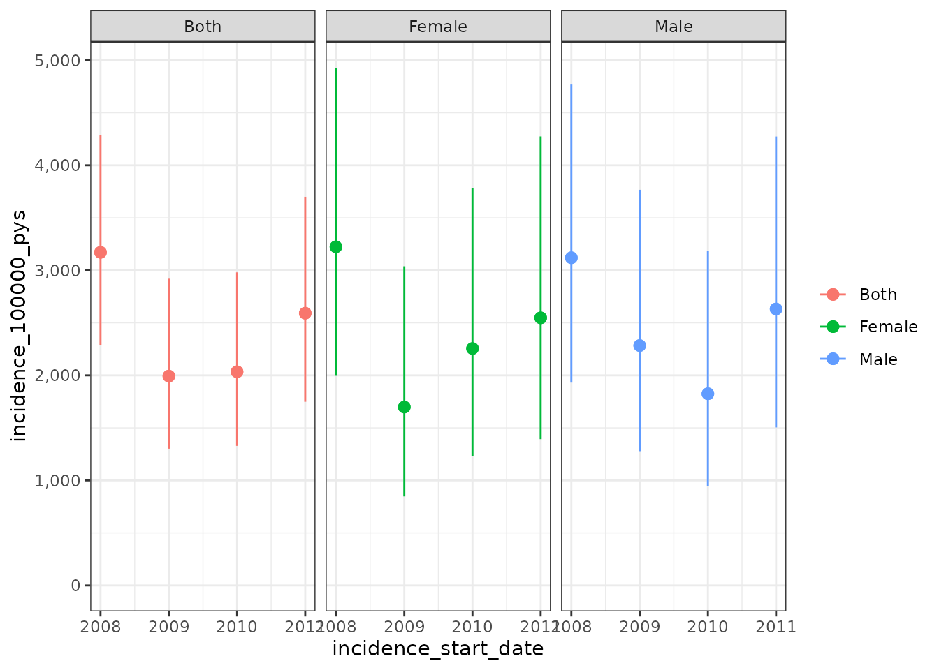
Similarly we can use the estimateIncidence() function to estimate incidence rates. Here we annual incidence rates, with 180 days used for outcome washout windows.

inc <- estimateIncidence(
  cdm = cdm,
  denominatorTable = "denominator",
  outcomeTable = "outcome",
  interval = c("Years"),
  outcomeWashout = 180
)

inc %>%
  glimpse()
#> Rows: 224
#> Columns: 13
#> $ result_id        <int> 1, 1, 1, 1, 1, 1, 1, 1, 1, 1, 1, 1, 1, 1, 1, 1, 1, 1,…
#> $ cdm_name         <chr> "mock", "mock", "mock", "mock", "mock", "mock", "mock…
#> $ group_name       <chr> "denominator_cohort_name &&& outcome_cohort_name", "d…
#> $ group_level      <chr> "denominator_cohort_3 &&& cohort_1", "denominator_coh…
#> $ strata_name      <chr> "overall", "overall", "overall", "overall", "overall"…
#> $ strata_level     <chr> "overall", "overall", "overall", "overall", "overall"…
#> $ variable_name    <chr> "Denominator", "Outcome", "Denominator", "Denominator…
#> $ variable_level   <chr> NA, NA, NA, NA, NA, NA, NA, NA, NA, NA, NA, NA, NA, N…
#> $ estimate_name    <chr> "denominator_count", "outcome_count", "person_days", …
#> $ estimate_type    <chr> "integer", "integer", "numeric", "numeric", "numeric"…
#> $ estimate_value   <chr> "1611", "42", "483778", "1324.512", "3170.979", "2285…
#> $ additional_name  <chr> "incidence_start_date &&& incidence_end_date &&& anal…
#> $ additional_level <chr> "2008-01-01 &&& 2008-12-31 &&& years", "2008-01-01 &&…