Plotting tools

visOmopResults offer some plotting tools that can be very useful. These tools are useful to plot either <summarised_result> dataset or a usual <data.frame>.

library(visOmopResults)

Plotting with a `<summarised_result>`

For the purpose of this vignette we will turn summarise the dataset penguins from the palmerpenguins package using PatientProfiles::summariseResult()

library(PatientProfiles)
library(palmerpenguins)
library(dplyr)
#> 
#> Attaching package: 'dplyr'
#> The following objects are masked from 'package:stats':
#> 
#>     filter, lag
#> The following objects are masked from 'package:base':
#> 
#>     intersect, setdiff, setequal, union

summariseIsland <- function(island) {
  penguins |>
    filter(.data$island == .env$island) |>
    summariseResult(
      group = "species",
      includeOverallGroup = TRUE,
      strata = list("year", "sex", c("year", "sex")),
      variables = c(
        "bill_length_mm", "bill_depth_mm", "flipper_length_mm", "body_mass_g", 
        "sex"),
      estimates = c(
        "median", "q25", "q75", "min", "max", "count_missing", "count", 
        "percentage", "density")
    ) |>
    suppressMessages() |>
    mutate(cdm_name = island)
}

penguinsSummary <- bind(
  summariseIsland("Torgersen"), 
  summariseIsland("Biscoe"), 
  summariseIsland("Dream")
)

Plotting principles

Although the input of a visOmopResult plot function can be a <summarised_result> when referring to inputs, we will use the columns shown in its tidy format:

tidyColumns(penguinsSummary)
#>  [1] "cdm_name"        "species"         "year"            "sex"            
#>  [5] "variable_name"   "variable_level"  "count"           "median"         
#>  [9] "q25"             "q75"             "min"             "max"            
#> [13] "count_missing"   "density_x"       "density_y"       "percentage"     
#> [17] "result_type"     "package_name"    "package_version"

And not the column names seen in the <summarised_result> format:

colnames(penguinsSummary)
#>  [1] "result_id"        "cdm_name"         "group_name"       "group_level"     
#>  [5] "strata_name"      "strata_level"     "variable_name"    "variable_level"  
#>  [9] "estimate_name"    "estimate_type"    "estimate_value"   "additional_name" 
#> [13] "additional_level"

That’s the most important thing to be aware of, otherwise populating arguments becomes a bit tricky.

We should always subset the <summarised_result> to the variable_name of interest before calling the plotting functions. It is not advised to combine results of different variables if they don’t share common estimates that we want to plot as in the tidy form NAs will be created.

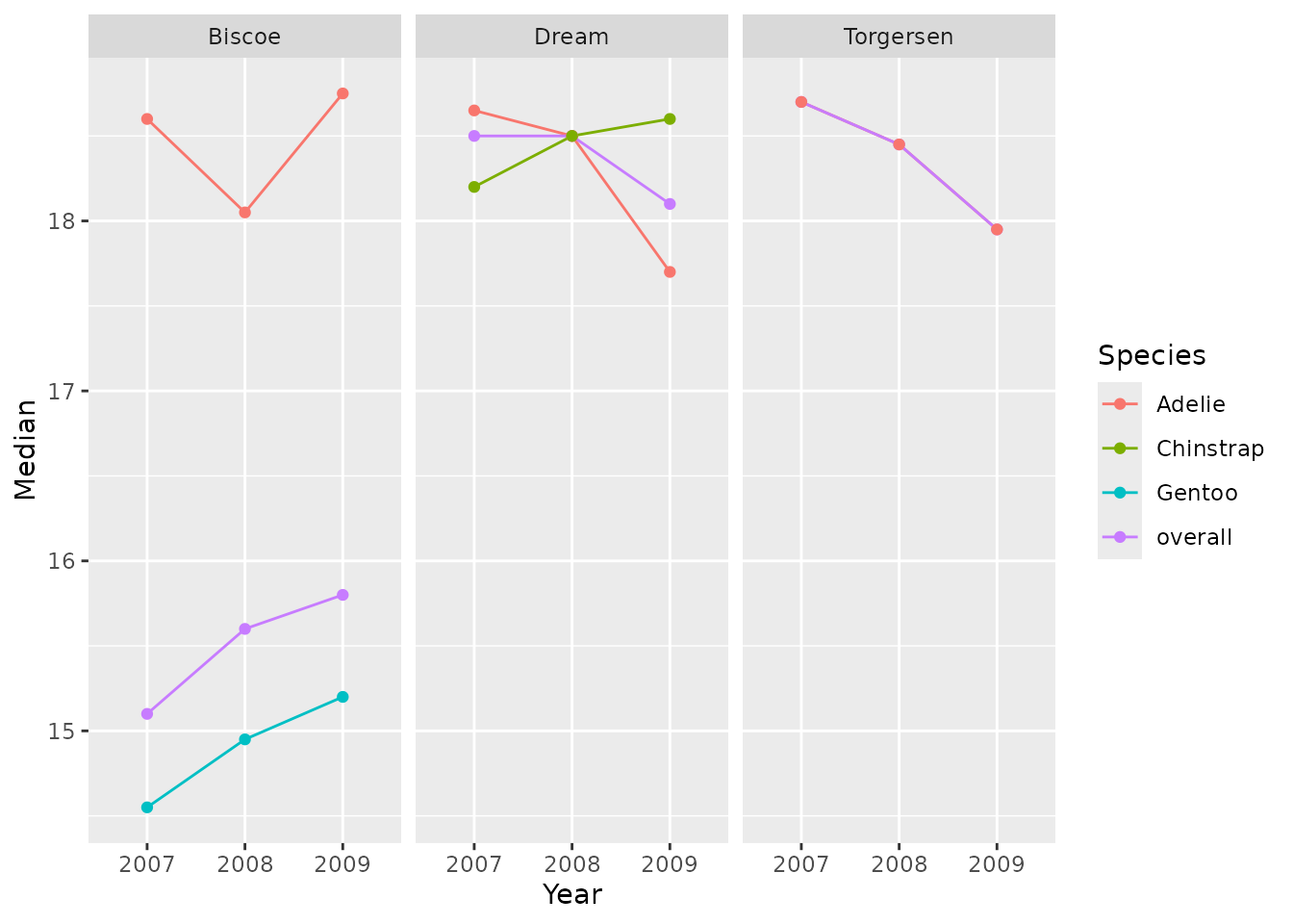
Scatter plot

We can create simple scatter plots using the plotScatter() let’s see some examples:

penguinsSummary |>
  filter(variable_name == "bill_depth_mm") |>
  filterStrata(year != "overall", sex == "overall") |>
  scatterPlot(
    x = "year", 
    y = "median",
    line = TRUE, 
    point = TRUE,
    ribbon = FALSE,
    facet = "cdm_name",
    colour = "species"
  )

penguinsSummary |>
  filter(variable_name %in% c("bill_length_mm", "bill_depth_mm"))|>
  filterStrata(year == "overall", sex == "overall") |>
  filterGroup(species != "overall") |>
  scatterPlot(
    x = "density_x", 
    y = "density_y",
    line = TRUE, 
    point = FALSE,
    ribbon = FALSE,
    facet = cdm_name ~ variable_name,
    colour = "species"
  ) +
  ggplot2::facet_grid(cdm_name ~ variable_name, scales = "free_x")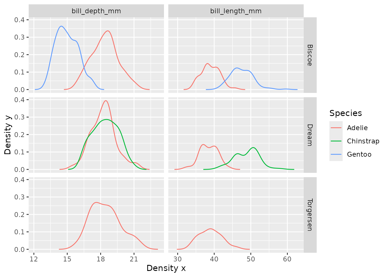

penguinsSummary |>
  filter(variable_name == "flipper_length_mm") |>
  filterStrata(year != "overall", sex %in% c("female", "male")) |>
  scatterPlot(
    x = c("year", "sex"), 
    y = "median",
    ymin = "q25",
    ymax = "q75",
    line = FALSE, 
    point = TRUE,
    ribbon = FALSE,
    facet = cdm_name ~ species,
    colour = "sex",
    group = c("year", "sex")
  ) +
  ggplot2::coord_flip() +
  ggplot2::labs(y = "Flipper length (mm)")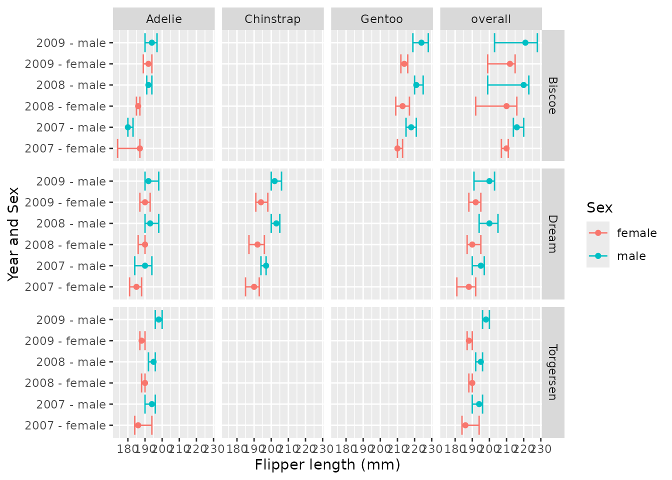

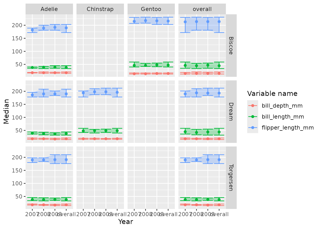
penguinsSummary |>
  filter(variable_name %in% c(
    "flipper_length_mm", "bill_length_mm", "bill_depth_mm")) |>
  filterStrata(sex == "overall") |>
  scatterPlot(
    x = "year", 
    y = "median",
    ymin = "min",
    ymax = "max",
    line = FALSE, 
    point = TRUE,
    ribbon = TRUE,
    facet = cdm_name ~ species,
    colour = "variable_name",
    group = c("variable_name")
  )

Bar plot

Let’s create some simple bar plots:

penguinsSummary |>
  filter(variable_name == "number records") |>
  filterGroup(species != "overall") |>
  filterStrata(sex != "overall", year != "overall") |>
  barPlot(
    x = "year",
    y = "count",
    colour = "sex",
    facet = cdm_name ~ species
  )

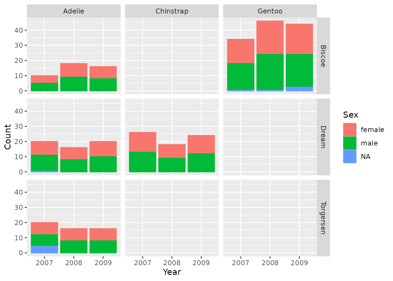
Box plot

Let’s create some box plots of their body mass:

penguinsSummary |>
  filter(variable_name == "body_mass_g") |>
  boxPlot(x = "year", facet = c("cdm_name", "species"), colour = "sex")

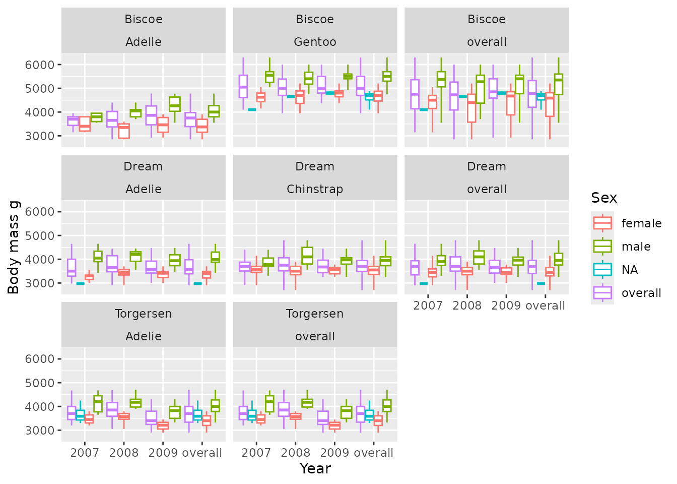
We can specify how we want to facet using a formula:

penguinsSummary |>
  filter(variable_name == "body_mass_g") |>
  boxPlot(x = "year", facet = cdm_name ~ species, colour = "sex")

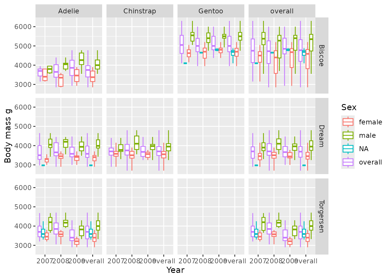
Arguments before ~ specify the rows, and arguments after the columns, see another example faceting also by sex in the columns. And in this case colouring by year:

penguinsSummary |>
  filter(variable_name == "body_mass_g") |>
  filterGroup(species != "overall") |>
  filterStrata(sex %in% c("female", "male"), year != "overall") |>
  boxPlot(facet = cdm_name ~ species + sex, colour = "year")

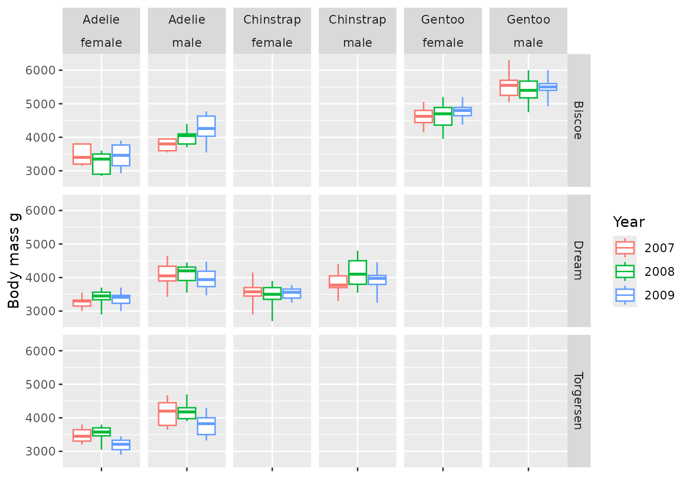
Note that as we didnt specify x there is no levels in the x axis, but box plots are produced anyway.

Plotting with a `<data.frame>`

Plotting functions can also be used with a normal <data.frame>. In this case we will use the tidy format of penguinsSummary.

penguinsTidy <- penguinsSummary |>
  filter(!estimate_name %in% c("density_x", "density_y")) |> # remove density for simplicity
  tidy()
penguinsTidy |> glimpse()
#> Rows: 720
#> Columns: 17
#> $ cdm_name        <chr> "Torgersen", "Torgersen", "Torgersen", "Torgersen", "T…
#> $ species         <chr> "overall", "overall", "overall", "overall", "overall",…
#> $ year            <chr> "overall", "overall", "overall", "overall", "overall",…
#> $ sex             <chr> "overall", "overall", "overall", "overall", "overall",…
#> $ variable_name   <chr> "number records", "bill_length_mm", "bill_depth_mm", "…
#> $ variable_level  <chr> NA, NA, NA, NA, NA, "female", "male", NA, NA, NA, NA, …
#> $ count           <int> 52, NA, NA, NA, NA, 24, 23, 5, 20, 16, 16, NA, NA, NA,…
#> $ median          <int> NA, 38, 18, 191, 3700, NA, NA, NA, NA, NA, NA, 38, 38,…
#> $ q25             <int> NA, 36, 17, 187, 3338, NA, NA, NA, NA, NA, NA, 37, 35,…
#> $ q75             <int> NA, 41, 19, 195, 4000, NA, NA, NA, NA, NA, NA, 39, 41,…
#> $ min             <int> NA, 33, 15, 176, 2900, NA, NA, NA, NA, NA, NA, 34, 33,…
#> $ max             <int> NA, 46, 21, 210, 4700, NA, NA, NA, NA, NA, NA, 46, 45,…
#> $ count_missing   <int> NA, 1, 1, 1, 1, NA, NA, NA, NA, NA, NA, 1, 0, 0, 1, 0,…
#> $ percentage      <dbl> NA, NA, NA, NA, NA, 46.153846, 44.230769, 9.615385, NA…
#> $ result_type     <chr> "summarise_table", "summarise_table", "summarise_table…
#> $ package_name    <chr> "PatientProfiles", "PatientProfiles", "PatientProfiles…
#> $ package_version <chr> "1.2.0", "1.2.0", "1.2.0", "1.2.0", "1.2.0", "1.2.0", …

That as it can be seen is a normal data.frame:

penguinsTidy |> class()
#> [1] "tbl_df"     "tbl"        "data.frame"

We can then do some custom plotting, for example replicating the last plot but from the tidy format:

penguinsTidy |>
  filter(
    variable_name == "body_mass_g",
    species != "overall",
    sex %in% c("female", "male"),
    year != "overall"
  ) |>
  boxPlot(facet = cdm_name ~ species + sex, colour = "year")

Custom plotting

The tidy format is very useful to apply any other custom ggplot2 function that we may be interested on:

library(ggplot2)
penguinsSummary |>
  filter(variable_name == "number records") |>
  tidy() |>
  ggplot(aes(x = year, y = sex, fill = count, label = count)) +
  geom_tile() +
  scale_fill_viridis_c(trans = "log") + 
  geom_text() +
  facet_grid(cdm_name ~ species)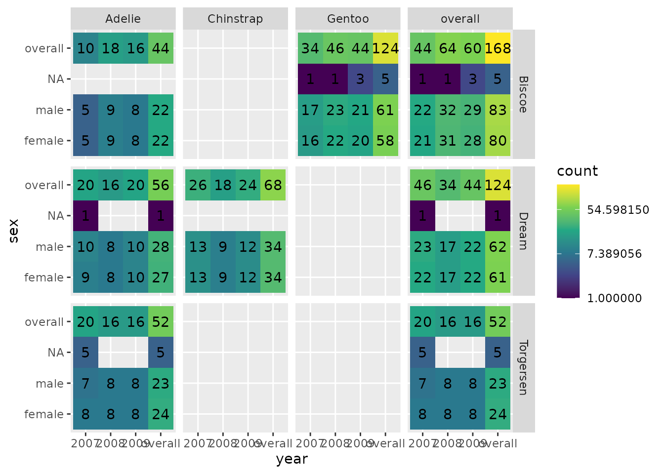

Combine with `ggplot2`

The plotting functions are a wrapper around the ggplot2 package, outputs of the plotting functions can be later customised with ggplot2 and similar tools. For example we can use ggplot2::labs() to change the labels and ggplot2::theme() to move the location of the legend.

penguinsSummary |>
  filter(
    group_level != "overall",
    strata_name == "year &&& sex",
    !grepl("NA", strata_level),
    variable_name == "body_mass_g") |>
  boxPlot(facet = cdm_name ~ species + sex, colour = "year") +
  ylim(c(0, 6500)) +
  labs(x = "My custom x label") +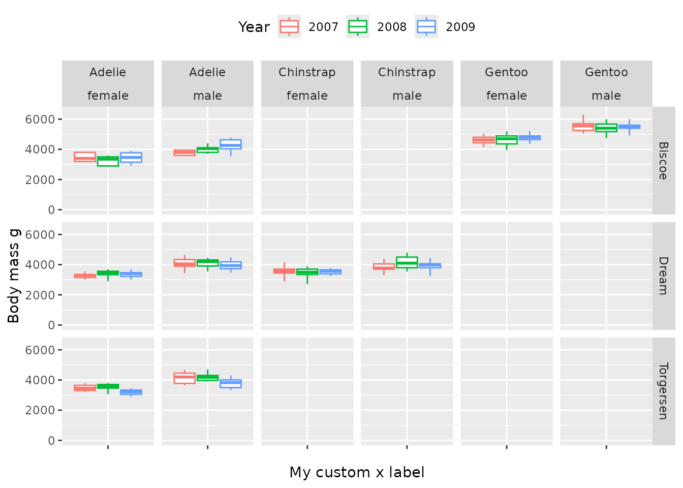
  theme(legend.position = "top")

You can also use ggplot2::ggsave() to later save one of this plots into ‘.png’ file.

ggsave(
  "figure8.png", plot = last_plot(), device = "png", width = 15, height = 12, 
  units = "cm", dpi = 300)

Combine with `plotly`

Although the package currently does not provide any plotly functionality ggplots can be easily converted to <plotly> ones using the function plotly::ggplotly(). This can make the interactivity of some plots better.

Plotting with a <summarised_result>